L02 · Performance & Power
Topic: intro · 41 pages
EECS 4340 Lecture 2 — Performance & Power
Announcements

Show slide text
Announcements
Labs start this Wednesday
- Please bring your computer
- Involve graded assignments
- Attendance is required and graded
Project #1
- Will be released today (26-Jan-26)
- Due 4-Feb-26
- More details in the lab
Recap: Fundamental concepts
Five key principles to performance
Show slide text
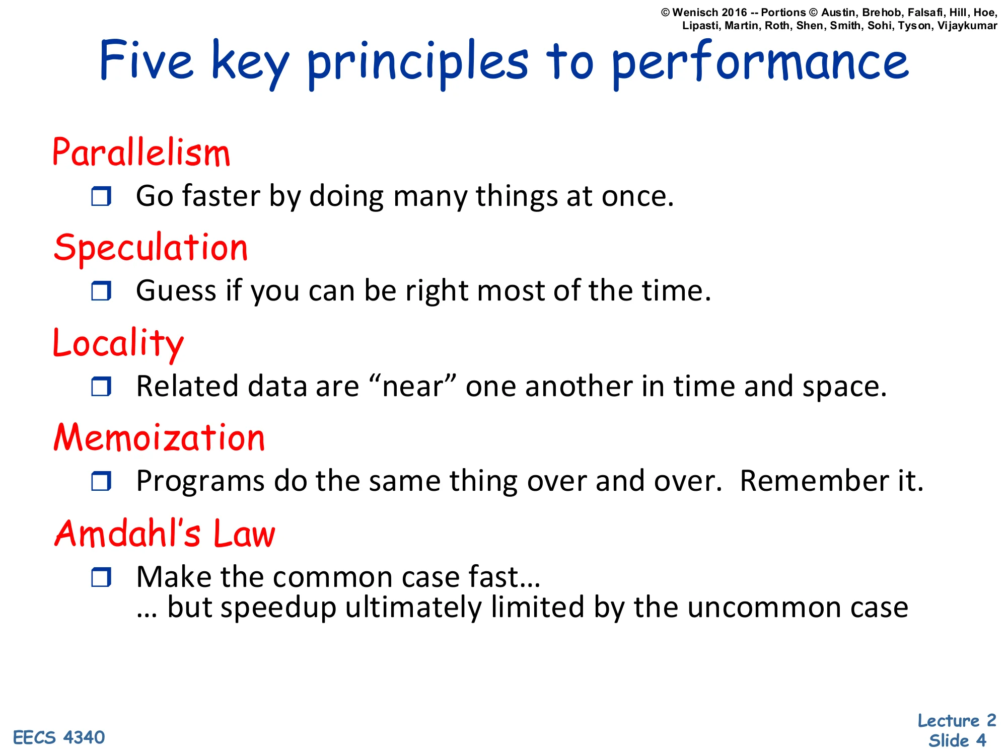
Five key principles to performance
Parallelism
- Go faster by doing many things at once.
Speculation
- Guess if you can be right most of the time.
Locality
- Related data are “near” one another in time and space.
Memoization
- Programs do the same thing over and over. Remember it.
Amdahl’s Law
- Make the common case fast…
- … but speedup ultimately limited by the uncommon case
This slide lays out the five recurring levers every later topic in EECS 4340 will pull. Parallelism covers everything from instruction-level parallelism in pipelines and out-of-order cores up to thread- and data-level parallelism in multiprocessors and SIMD. Speculation covers branch prediction, value prediction, and speculative memory disambiguation — fetch and execute past unresolved events on the bet that you’ll be right and squash on misprediction. Locality underpins the entire memory hierarchy: temporal locality (recently-used data will be reused) and spatial locality (nearby addresses will be touched soon) are why caches and prefetchers work. Memoization is the conceptual umbrella for caching results — caches, TLBs, branch target buffers, even register renaming maps are all memoizations. Amdahl’s Law is the meta-principle that constrains all of the above: optimize the common case, but understand that the un-optimized fraction sets a hard floor on overall speedup, so you can’t ignore it forever.
Amdahl's Law
Show slide text
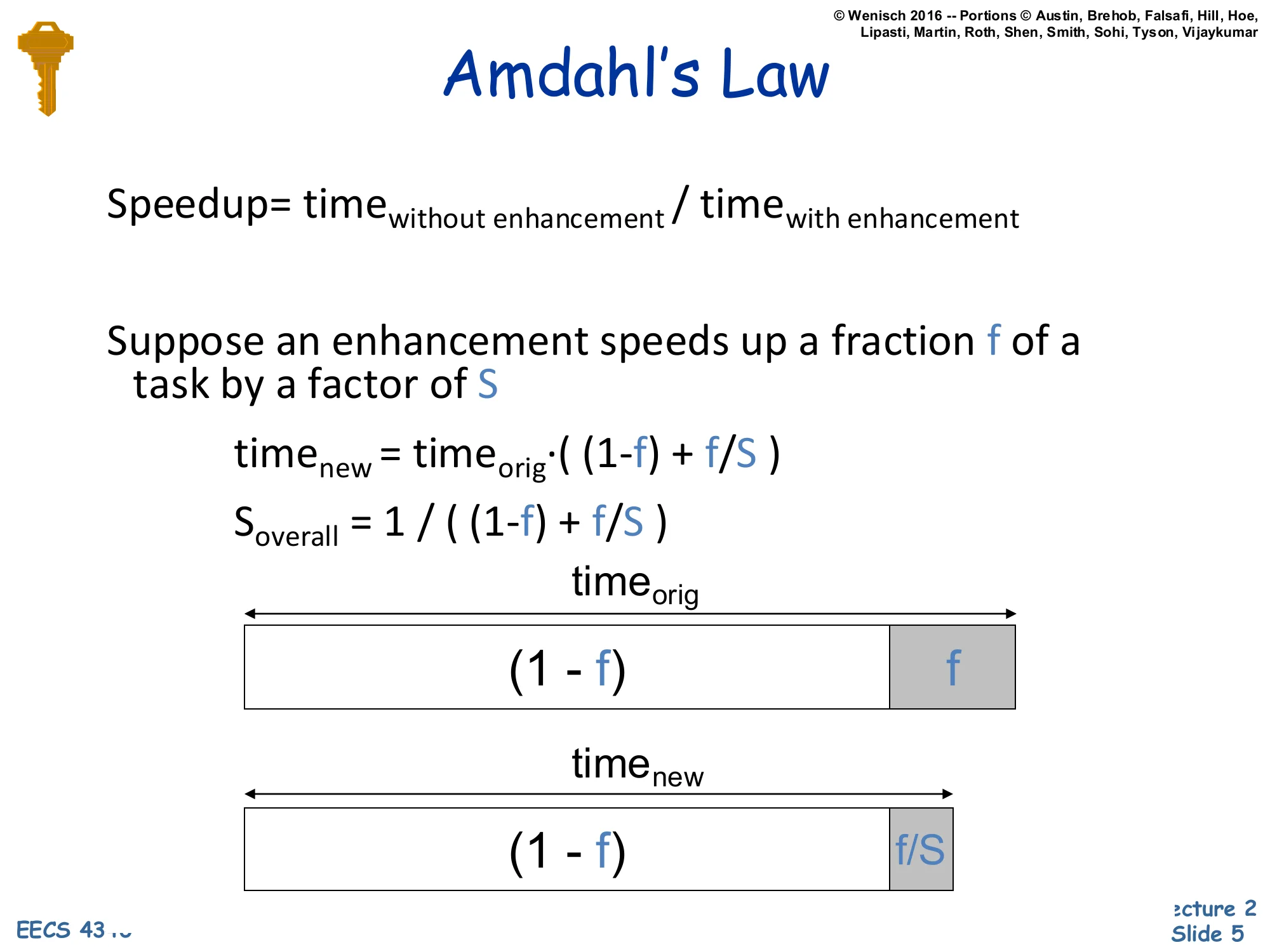
Amdahl’s Law
Speedup=timewith enhancementtimewithout enhancement
Suppose an enhancement speeds up a fraction f of a task by a factor of S
timenew=timeorig⋅((1−f)+Sf)
Soverall=(1−f)+f/S1
(Bar diagram: timeorig split into (1−f) and f; timenew split into (1−f) and f/S.)
Amdahl’s Law quantifies the speedup ceiling for a partial optimization. Take an original task of unit time and split it into the fraction f that the enhancement accelerates and the fraction (1−f) that it does not. After the enhancement, the unaffected portion still takes (1−f) and the accelerated portion shrinks from f to f/S, where S is the local speedup. Total new time is the sum, and overall speedup is 1/((1−f)+f/S).
Two limit checks build intuition. If S→∞ (the enhanced part becomes free), overall speedup approaches 1/(1−f) — bounded by the un-enhanced fraction. If f is small, even a huge S barely moves the needle. This is why microarchitects obsess over which slices of execution time their proposed feature actually accelerates: a 100x improvement on a 1% slice yields just 1.01x overall. The bar diagram on the slide is the classic visualization — the (1−f) block is fixed in width while the f block compresses to f/S, and the overall ratio is the ratio of the bar lengths.
Measuring performance
Performance
Show slide text
Performance
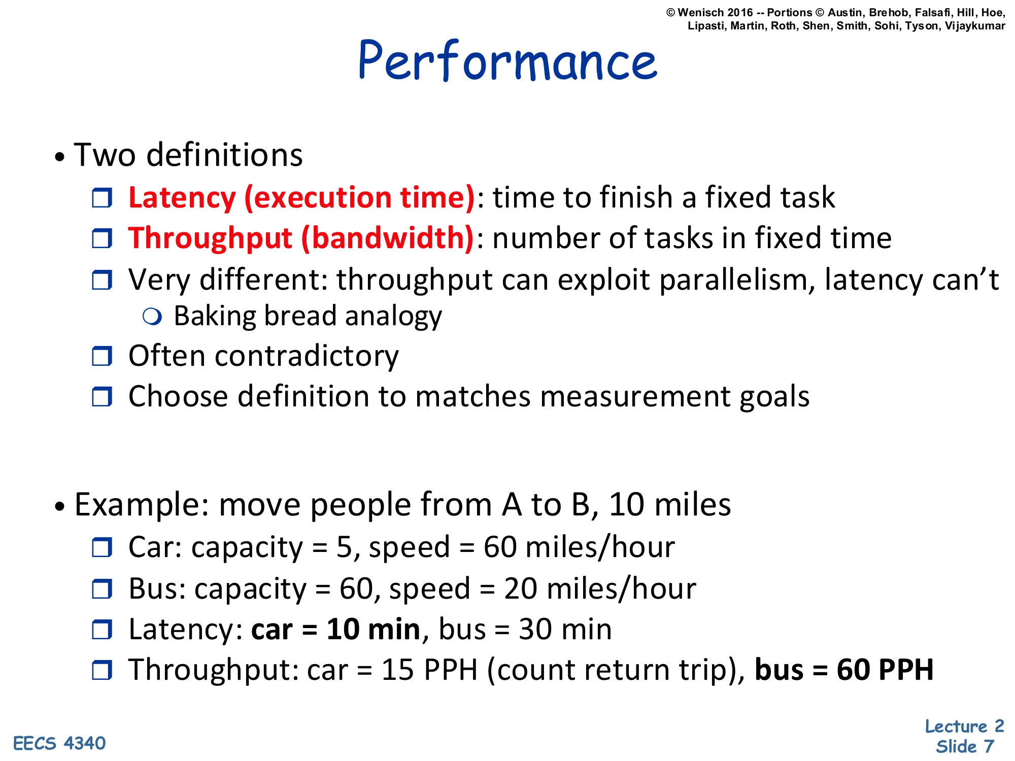
- Two definitions
- Latency (execution time): time to finish a fixed task
- Throughput (bandwidth): number of tasks in fixed time
- Very different: throughput can exploit parallelism, latency can’t
- Baking bread analogy
- Often contradictory
- Choose definition to matches measurement goals
- Example: move people from A to B, 10 miles
- Car: capacity = 5, speed = 60 miles/hour
- Bus: capacity = 60, speed = 20 miles/hour
- Latency: car = 10 min, bus = 30 min
- Throughput: car = 15 PPH (count return trip), bus = 60 PPH
Performance has two non-interchangeable definitions, and confusing them is one of the most common bugs in architecture papers. Latency is how long one fixed task takes — relevant when you care about a single user-visible operation completing. Throughput is how many tasks finish per unit time — relevant when you care about aggregate work like a webserver’s request rate or a datacenter’s queries-per-second. The two are very different because throughput can be improved by parallelism (run many tasks in parallel) while latency for a single serial task cannot — adding more bakers does not let one loaf of bread bake any faster, but it does let you produce more loaves per hour.
The car-vs-bus example shows the contradiction directly. The car covers 10 miles in 10 minutes, the bus in 30 minutes — so the car wins on latency by 3x. But if you count the round trip (car must return to pick up the next group), the bus moves 60 people per hour while the car moves only 15 — the bus wins on throughput by 4x. Choose the metric that matches what your customer is actually paying for.
Performance Improvement
Show slide text
Performance Improvement
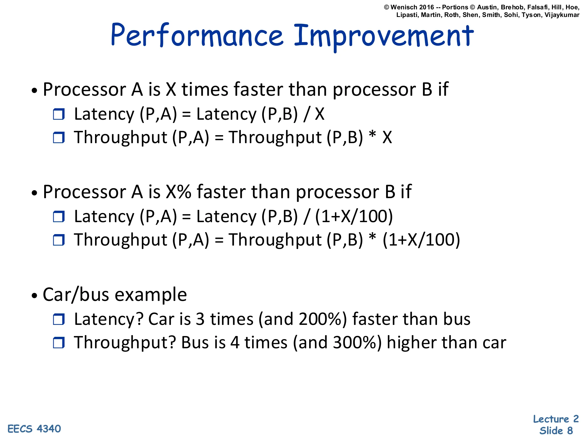
- Processor A is X times faster than processor B if
- Latency(P,A)=Latency(P,B)/X
- Throughput(P,A)=Throughput(P,B)⋅X
- Processor A is X% faster than processor B if
- Latency(P,A)=Latency(P,B)/(1+X/100)
- Throughput(P,A)=Throughput(P,B)⋅(1+X/100)
- Car/bus example
- Latency? Car is 3 times (and 200%) faster than bus
- Throughput? Bus is 4 times (and 300%) higher than car
This slide pins down the language used to compare two designs. Saying “A is X times faster than B” is a multiplicative claim: A’s latency is B’s divided by X, equivalently A’s throughput is B’s multiplied by X. Saying “A is X% faster” is a percentage claim: divide latency by (1+X/100) or multiply throughput by the same factor. The two statements are not equivalent — “3 times faster” corresponds to a 200% improvement, not 300%, because the baseline (1×) is already counted. The car-vs-bus row makes this explicit: if the car’s latency is one third of the bus’s, the car is 3 times faster and 200% faster (since 3=1+200/100). The bus has 4× the car’s throughput, equivalently 300% higher. Many casual benchmark write-ups conflate these two and overstate improvements; getting the convention right is a basic professional skill.
Averaging Performance Numbers I
Show slide text
Averaging Performance Numbers I
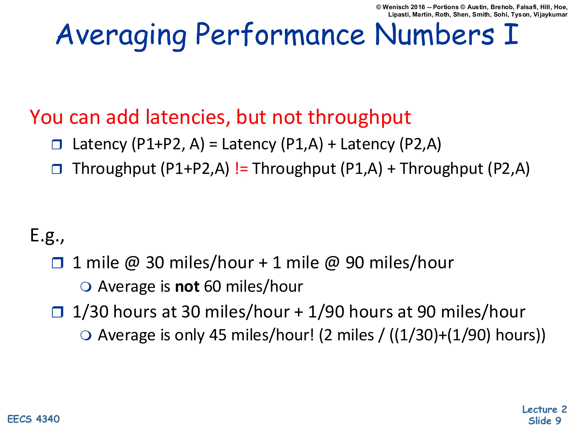
You can add latencies, but not throughput
- Latency(P1+P2,A)=Latency(P1,A)+Latency(P2,A)
- Throughput(P1+P2,A)=Throughput(P1,A)+Throughput(P2,A)
E.g.,
- 1 mile @ 30 miles/hour + 1 mile @ 90 miles/hour
- Average is not 60 miles/hour
- 1/30 hours at 30 miles/hour + 1/90 hours at 90 miles/hour
- Average is only 45 miles/hour! (2 miles/((1/30)+(1/90)) hours)
This is the most-tested gotcha on early problem sets. Latencies compose by addition: total time on a sequence of programs is the sum of times. Throughput does not compose by addition because throughput is a rate (instructions per second, miles per hour, queries per second), and rates depend on which time interval you average over.
The slide’s example is the canonical trap. Drive one mile at 30 mph, then one mile at 90 mph. The naive arithmetic mean of speeds is 60 mph. But the actual average speed (total distance over total time) is 2/(1/30+1/90)=2/(4/90)=45 mph. Why? You spend much more time in the slow segment than the fast one, so it dominates the average. The correct average of two rates over equal distances is the harmonic mean: 1/r1+1/r22. Over equal times it would be the arithmetic mean. The next slide formalizes when each averaging technique applies.
Averaging Performance Numbers II
Show slide text
Averaging Performance Numbers II
-
Latency(P1+P2,A)=Latency(P1,A)+Latency(P2,A)
-
Throughput(P1+P2,A)=Throughput(P1,A)1+Throughput(P2,A)11
-
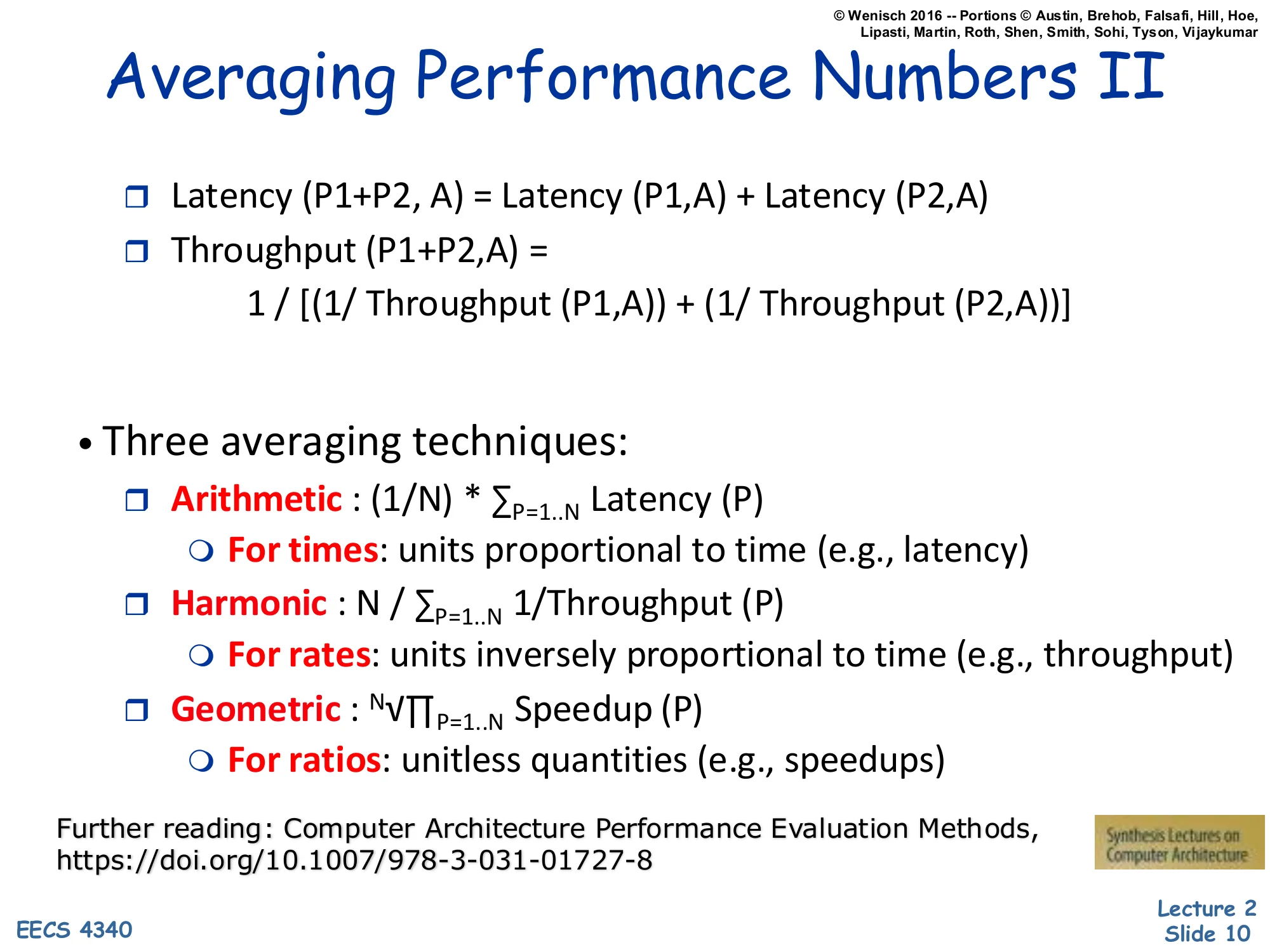
Three averaging techniques:
- Arithmetic: (1/N)⋅∑P=1..NLatency(P)
- For times: units proportional to time (e.g., latency)
- Harmonic: N/∑P=1..N1/Throughput(P)
- For rates: units inversely proportional to time (e.g., throughput)
- Geometric: N∏P=1..NSpeedup(P)
- For ratios: unitless quantities (e.g., speedups)
- Arithmetic: (1/N)⋅∑P=1..NLatency(P)
Further reading: Computer Architecture Performance Evaluation Methods, https://doi.org/10.1007/978-3-031-01727-8
Three averaging techniques cover three distinct measurement types. Arithmetic mean, xˉ=N1∑xi, is correct when the quantity is proportional to time — execution times, latencies, cycles. Harmonic mean, xˉ=N/∑(1/xi), is correct for rates (instructions per second, MIPS, bandwidth) because the harmonic mean of rates equals the arithmetic mean of the underlying times. Geometric mean, xˉ=N∏xi, is the correct mean for normalized ratios such as speedup vs a baseline; it is the unique mean that is independent of which machine you choose as the reference, so SPEC ratings use it.
The right-hand identity also shows that throughput composes by harmonic addition: when running two programs sequentially, total throughput follows 1/(1/T1+1/T2), not T1+T2. Picking the wrong mean is one of the most common mistakes in published benchmarks; the further reading link points to a Synthesis Lectures monograph that walks through dozens of examples.
The "Iron Law" of Processor Performance
Show slide text
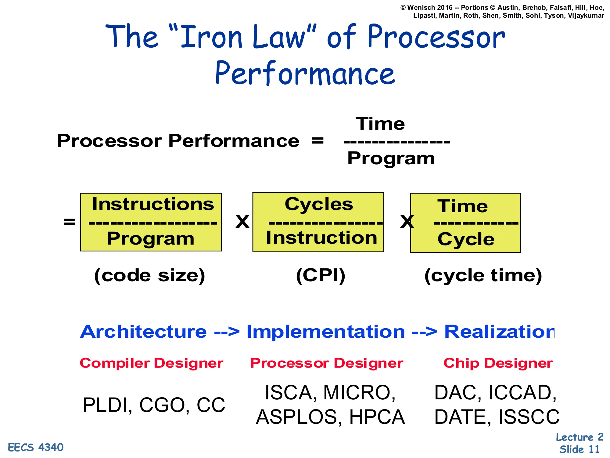
The “Iron Law” of Processor Performance
Processor Performance=ProgramTime=ProgramInstructions×InstructionCycles×CycleTime
(code size) × (CPI) × (cycle time)
Architecture → Implementation → Realization
| Compiler Designer | Processor Designer | Chip Designer |
|---|---|---|
| PLDI, CGO, CC | ISCA, MICRO, ASPLOS, HPCA | DAC, ICCAD, DATE, ISSCC |
The Iron Law decomposes wall-clock execution time per program into three multiplicative factors: dynamic instruction count (instructions per program), cycles per instruction, and cycle time (seconds per cycle). Every architectural choice affects exactly one — or sometimes trades one against another — of these three terms, and naming the term you’re targeting is the first step in any serious design discussion.
The slide also maps each factor to the community responsible for it. The instruction count is the compiler designer’s territory — choose a denser ISA encoding or a smarter optimization pass and the dynamic instruction count drops; the relevant venues are PLDI, CGO, and CC. CPI is the processor designer’s domain — pipelining, out-of-order execution, branch prediction, and caches all change how many cycles each instruction takes on average; the venues are ISCA, MICRO, ASPLOS, and HPCA. Cycle time is the chip designer’s job — circuit techniques, layout, process choice; the venues are DAC, ICCAD, DATE, and ISSCC. The lecture’s later topics will mostly target the middle column.
Danger: Partial Performance Metrics
Show slide text
Danger: Partial Performance Metrics
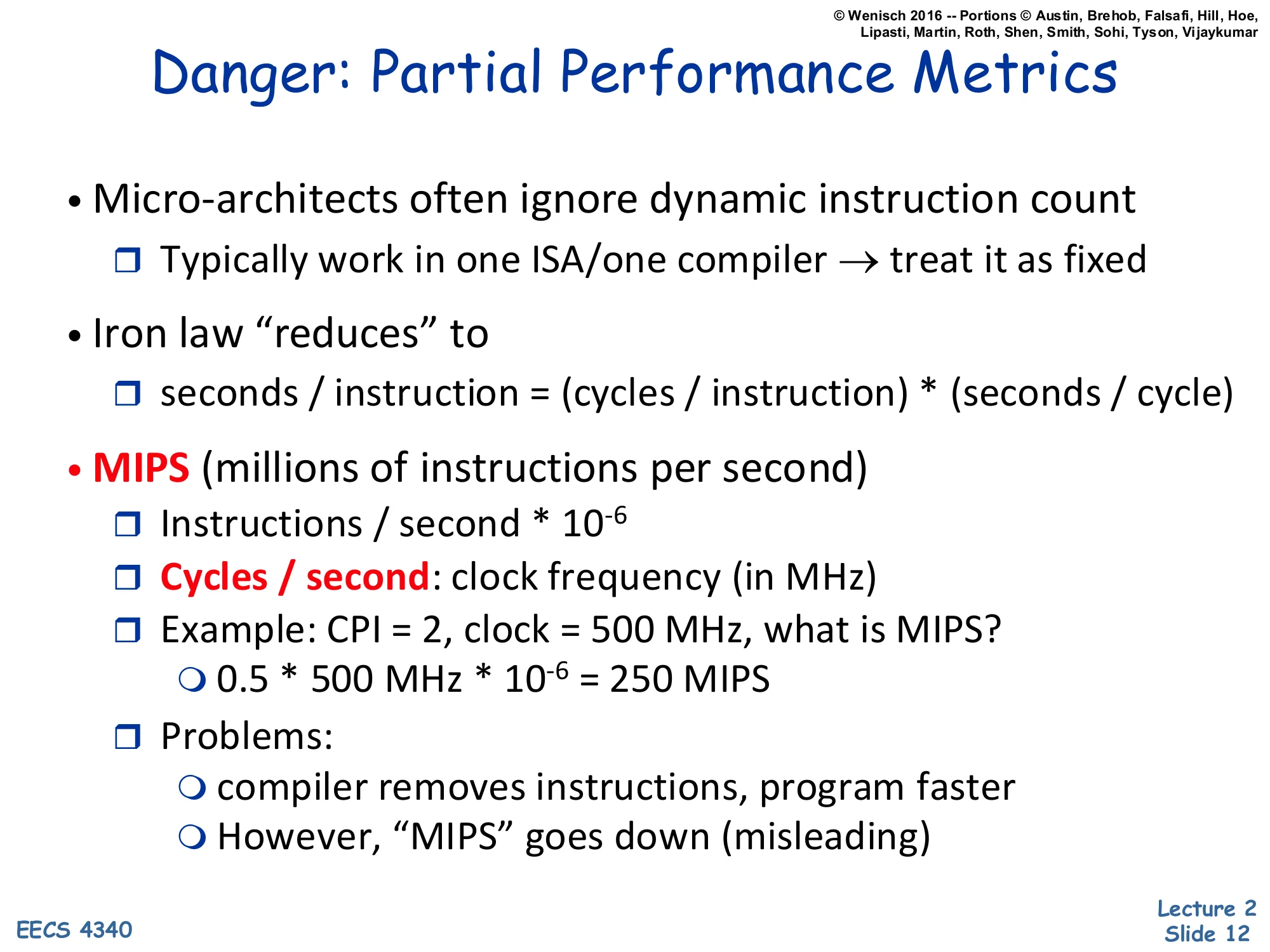
- Micro-architects often ignore dynamic instruction count
- Typically work in one ISA/one compiler → treat it as fixed
- Iron law “reduces” to
- seconds / instruction = (cycles / instruction) × (seconds / cycle)
- MIPS (millions of instructions per second)
- Instructions / second × 10−6
- Cycles / second: clock frequency (in MHz)
- Example: CPI = 2, clock = 500 MHz, what is MIPS?
- 0.5×500 MHz×10−6=250 MIPS
- Problems:
- compiler removes instructions, program faster
- However, “MIPS” goes down (misleading)
Micro-architects rarely change the ISA or the compiler in a single project, so they treat the instruction-count term as fixed and reason about seconds-per-instruction = CPI × cycle time. That simplification is fine inside a project but dangerous when comparing across them — change the compiler and you can break this assumption silently.
MIPS is the most cited reduced metric: instructions per second divided by 106, equivalently clock frequency in MHz divided by CPI. The worked example shows CPI = 2 at 500 MHz gives 500/2=250 MIPS. The problem is that MIPS rewards executing many cheap instructions even when the program does less actual work — a smarter compiler that removes instructions makes the program faster (less wall-clock time) but can simultaneously make MIPS lower (fewer instructions per second), because the remaining instructions are harder. Hence the famous quip that MIPS stands for “Meaningless Indicator of Performance for Salespeople.”
Danger: Partial Performance Metrics II
Show slide text
Danger: Partial Performance Metrics II
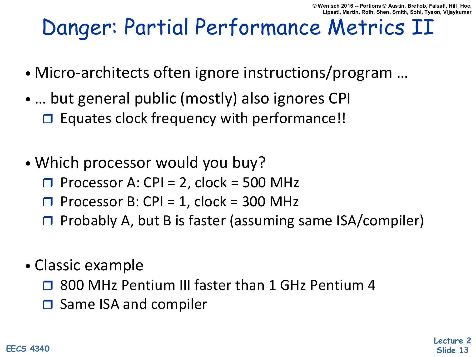
- Micro-architects often ignore instructions/program …
- … but general public (mostly) also ignores CPI
- Equates clock frequency with performance!!
- Which processor would you buy?
- Processor A: CPI = 2, clock = 500 MHz
- Processor B: CPI = 1, clock = 300 MHz
- Probably A, but B is faster (assuming same ISA/compiler)
- Classic example
- 800 MHz Pentium III faster than 1 GHz Pentium 4
- Same ISA and compiler
If architects err by ignoring instruction count, the buying public errs by ignoring CPI: they read “3 GHz” off a spec sheet and equate frequency with performance. The slide’s worked example shows why this is wrong. Processor A runs at 500 MHz with CPI = 2, so it completes 250 million instructions per second. Processor B runs at only 300 MHz but with CPI = 1, completing 300 million instructions per second — 20% faster despite the slower clock. The Iron Law makes this obvious: time=IC×CPI×Tcycle, and CPI and frequency multiply.
The Pentium III vs Pentium 4 row is the canonical real-world example. Intel’s NetBurst architecture (Pentium 4) used a very deep pipeline to hit high clock frequencies, but the deep pipeline raised CPI dramatically due to mispredicted branches and cache misses. An 800 MHz Pentium III with much better CPI beat a 1 GHz Pentium 4 on most integer code. Frequency is a marketing number; what matters is the product of all three Iron Law terms.
Performance — Key Points
Show slide text
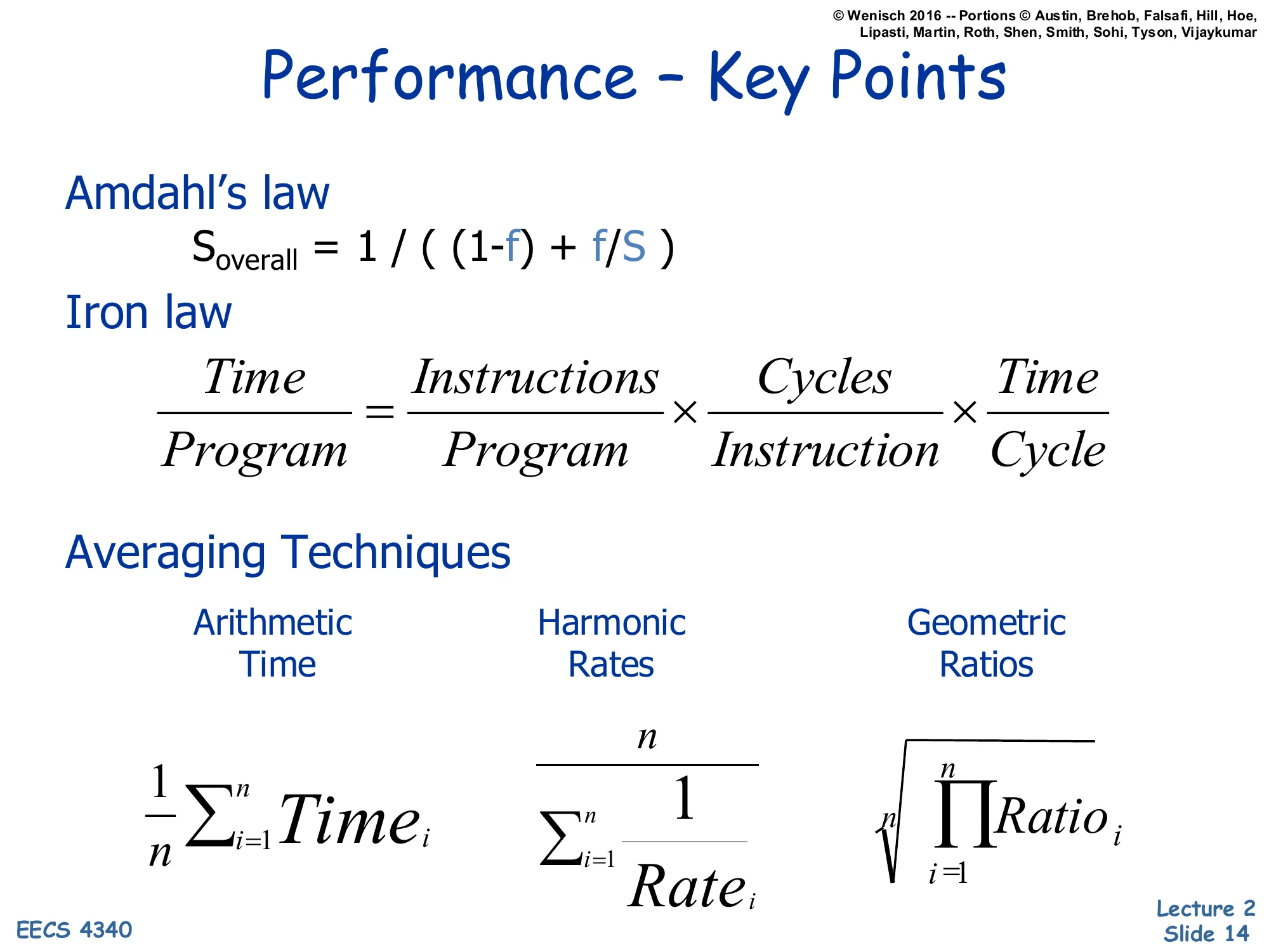
Performance — Key Points
Amdahl’s law
Soverall=(1−f)+f/S1
Iron law
ProgramTime=ProgramInstructions×InstructionCycles×CycleTime
Averaging Techniques
- Arithmetic (Time): n1∑i=1nTimei
- Harmonic (Rates): ∑i=1nRatei1n
- Geometric (Ratios): n∏i=1nRatioi
This is the consolidated performance summary you should be able to recite without notes by exam time. Three formulas, each owning a distinct slice of the design space.
Amdahl’s law gives you the speedup ceiling for any partial enhancement: if only fraction f of execution is improved by factor S, total speedup is bounded by 1/((1−f)+f/S), which approaches 1/(1−f) as S→∞. Use it to sanity-check whether a proposed optimization is worth implementing.
The Iron Law decomposes execution time per program into three multiplicative factors — dynamic instruction count, CPI, and cycle time — and assigns responsibility for each to compiler, microarchitect, and circuit designer respectively. Every architectural change should be analyzable as a tradeoff among these three terms.
The averaging techniques tell you which mean to take when summarizing across many measurements: arithmetic for raw times, harmonic for rates, geometric for normalized ratios. Picking the wrong one will silently distort conclusions.
Power

Why care about Power & Energy?
Show slide text
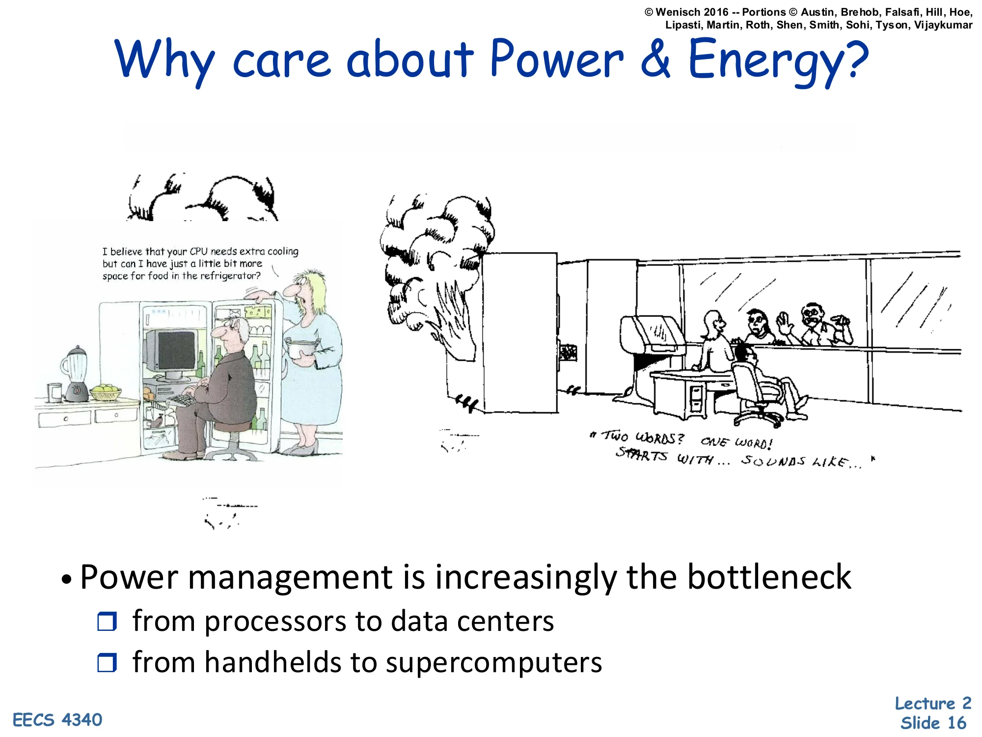
Why care about Power & Energy?
(Cartoons: a CPU needing extra cooling so a kitchen has “a little bit less space for food in the refrigerator,” and a smoking PC; “two words: one wall starts with… sounds like…”)
- Power management is increasingly the bottleneck
- from processors to data centers
- from handhelds to supercomputers
This slide motivates the entire second half of the lecture. From the late 1990s through the early 2000s, processor designers chased clock frequency aggressively, and CPUs went from a few watts to over 100 watts in roughly a decade. The cartoons are a visual gag: PCs eventually needed cooling solutions so large they competed with kitchen appliances, and overclocked machines literally burned out.
The takeaway is that power management is now the dominant constraint, not raw transistor count or clock speed. Mobile devices are limited by battery capacity and skin temperature. Datacenters are limited by total facility power, cooling capacity, and electricity bills. Even supercomputers like exascale machines are budgeted in megawatts before they are budgeted in FLOPs. This shifted the entire field — pre-2005 architecture papers cared mostly about IPC, post-2005 papers always report performance-per-watt. The rest of L02 builds the vocabulary for analyzing power tradeoffs.
Power vs. Energy
Show slide text
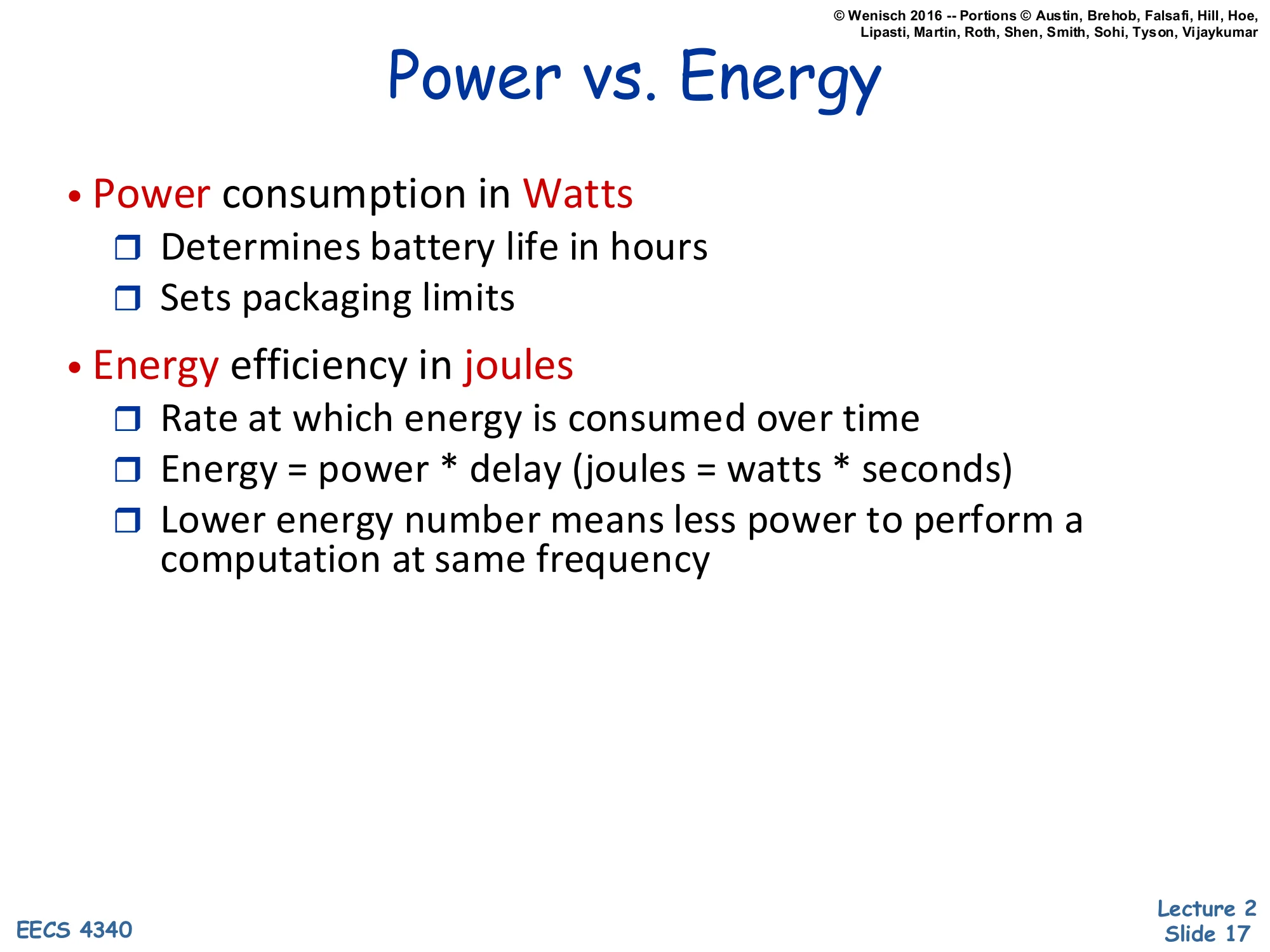
Power vs. Energy
- Power consumption in Watts
- Determines battery life in hours
- Sets packaging limits
- Energy efficiency in joules
- Rate at which energy is consumed over time
- Energy = power × delay (joules = watts × seconds)
- Lower energy number means less power to perform a computation at same frequency
Power and energy are easy to confuse in casual speech but mean different things and bind different constraints. Power is the instantaneous rate of energy consumption, measured in watts (joules per second). It dictates instantaneous things like how hot the chip gets, how big the heatsink must be, and how much current the voltage regulator must deliver. Energy is the time integral of power, measured in joules. It dictates accumulating things like total electricity used, total heat dumped, and how long a battery lasts.
The relation Energy=Power×Time couples them, but the implications differ. A laptop’s battery life depends on energy used during the workload. A laptop’s package and fan are sized for peak power. A design that finishes a fixed task with less energy is genuinely more efficient — it accomplishes the same computation while drawing less from the battery. Note that the slide says “rate at which energy is consumed over time” under “Energy”; in standard usage that phrase actually defines power, but this slide uses it loosely to introduce the joule unit.
The distinction motivates the combined metrics (PDP, EDP, ED²P) introduced later in the lecture.
Power vs. Energy (graphical)
Show slide text
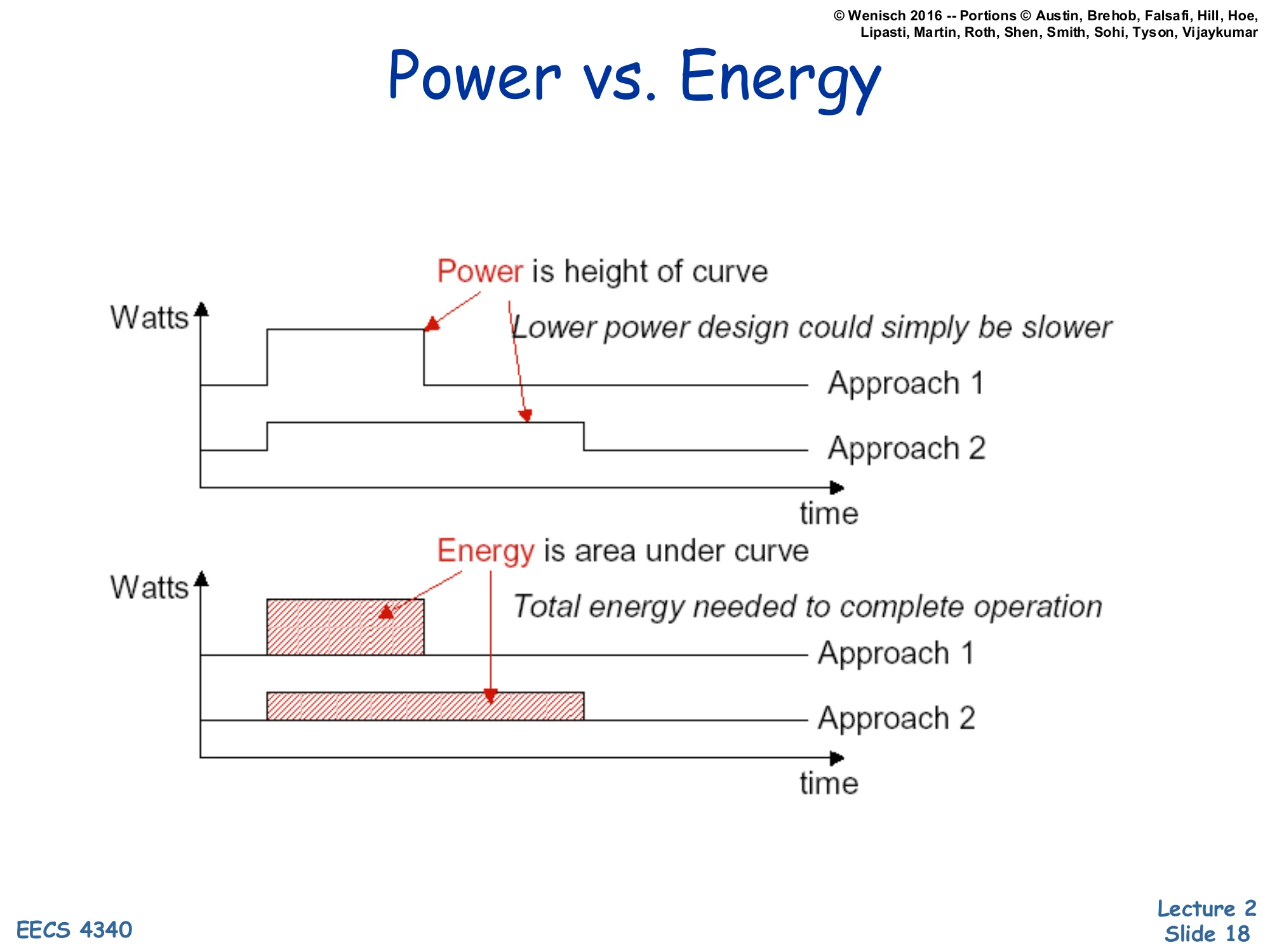
Power vs. Energy
Top chart (Watts vs. time):
- Power is height of curve
- Lower power design could simply be slower
- Approach 1: high, short bar
- Approach 2: lower, longer bar
Bottom chart (Watts vs. time):
- Energy is area under curve
- Total energy needed to complete operation
- Approach 1 area vs. Approach 2 area
The two stacked plots make the power/energy distinction visual. In the top plot the y-axis is power (watts) and the x-axis is time. Approach 1 finishes the same task quickly but at a high power level (a tall, short rectangle). Approach 2 finishes the same task more slowly at a lower power level (a shorter, longer rectangle). The height of each rectangle is power — Approach 2 wins the “lower watts” comparison.
In the bottom plot the area under each curve is energy = power × time. The takeaway is that Approach 2’s lower peak power doesn’t automatically mean lower energy; if it runs proportionally longer, the areas can be equal or even reversed. A design that simply throttles down (lower V, lower f, longer runtime) can deliver lower peak power without saving energy — and if static (leakage) power keeps flowing during the longer runtime, total energy can actually increase. This is the central tension behind the “race to halt” strategy used in modern mobile CPUs: finish fast at high power, then deep-sleep, often beating sustained low-power operation on total energy.
Breakout Room Discussion
Show slide text
Breakout Room Discussion
- 5 Minutes
- Introduce yourselves to one another
- Come up with examples of systems that might be energy constrained (and why) as well as some that might be power constrained (and why).
An in-class group exercise. Energy-constrained systems are those whose total runtime is limited by a finite stored-energy budget — phones, laptops, sensor motes, electric vehicles, satellites. For these, what matters is joules per task: minimize the integral of power over the workload, even if that means higher peak watts for short bursts. Power-constrained systems are those limited by an instantaneous heat or current ceiling — datacenter racks (limited by PDU amps and rack cooling), server CPUs (limited by socket TDP and heatsink capacity), and chip packages themselves (limited by what the silicon can dissipate before exceeding Tj specifications). These systems care about peak watts even if total energy over a year is less interesting because grid power is essentially infinite. A useful exam test: “is the limit a battery or a cooling solution?” — battery means energy, cooling means power.
Why is energy important?
Show slide text
Why is energy important?
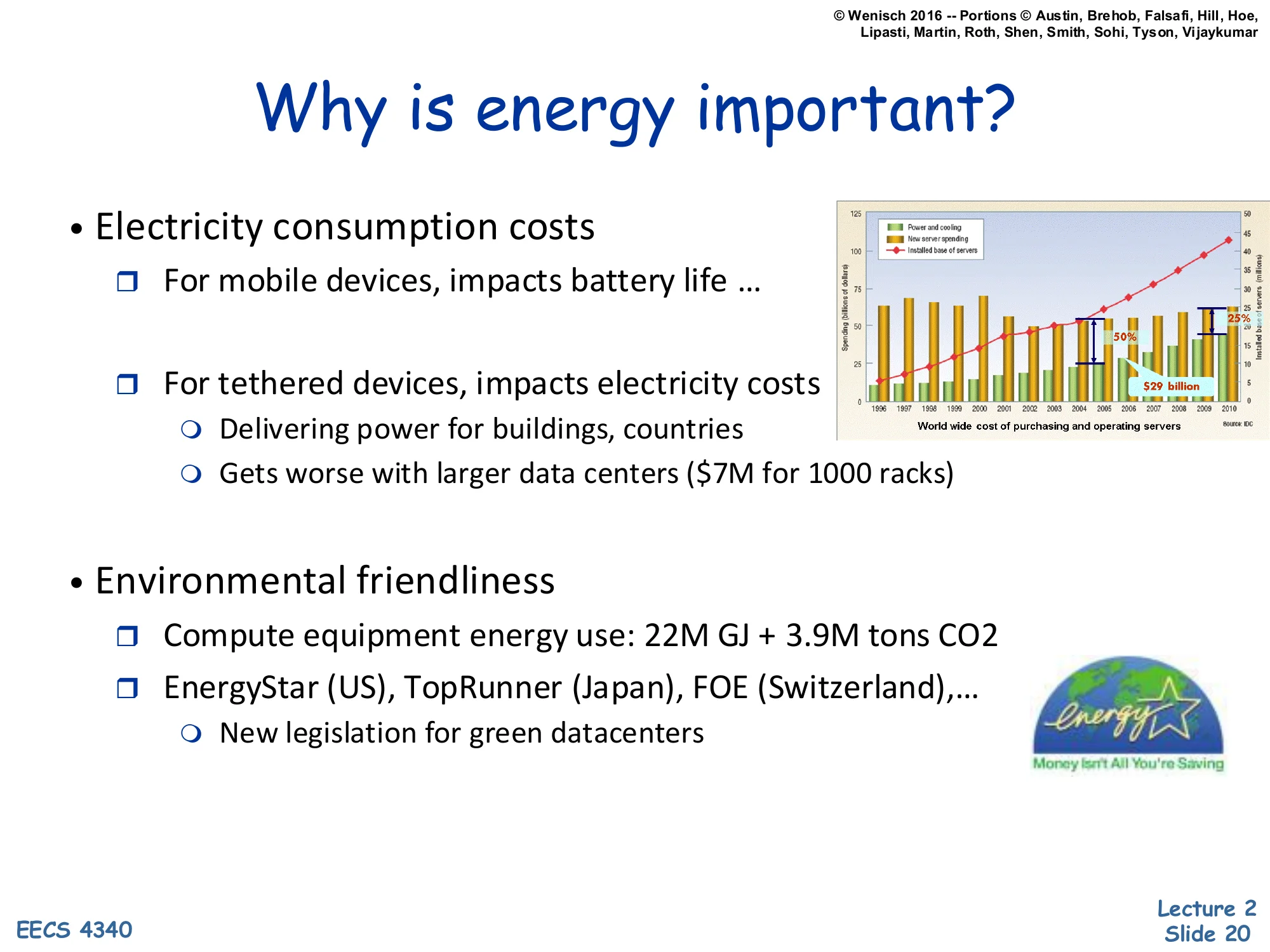
- Electricity consumption costs
- For mobile devices, impacts battery life …
- For tethered devices, impacts electricity costs
- Delivering power for buildings, countries
- Gets worse with larger data centers ($7M for 1000 racks)
- Environmental friendliness
- Compute equipment energy use: 22M GJ + 3.9M tons CO2
- EnergyStar (US), TopRunner (Japan), FOE (Switzerland), …
- New legislation for green datacenters
(Right: bar chart of worldwide cost of purchasing and operating servers, with operating cost crossing purchasing cost; “$3B billion”.)
Energy matters at three scales. At the device scale, mobile users notice battery life directly — every joule saved extends runtime. At the facility scale, datacenters pay enormous electricity bills: the slide cites $7 million for a thousand-rack site, which is plausible at typical commercial rates and rack power densities. The right-hand bar chart shows that worldwide server operating costs (mostly electricity for power and cooling) eventually crossed purchasing costs around the mid-2000s — meaning a server’s lifetime electricity bill exceeds the purchase price. That crossover changed datacenter design priorities: efficiency improvements pay back faster than buying cheaper hardware.
At the global scale, computing equipment accounts for tens of millions of GJ of energy and millions of tons of CO₂ annually. Regulatory programs — EnergyStar in the US, TopRunner in Japan, FOE in Switzerland — push manufacturers to disclose and reduce energy use, and several jurisdictions now have explicit “green datacenter” legislation. So energy efficiency is simultaneously an engineering metric, a financial metric, and a regulatory metric — three distinct stakeholders all pulling the same direction.
Why is power important?
Show slide text
Why is power important?
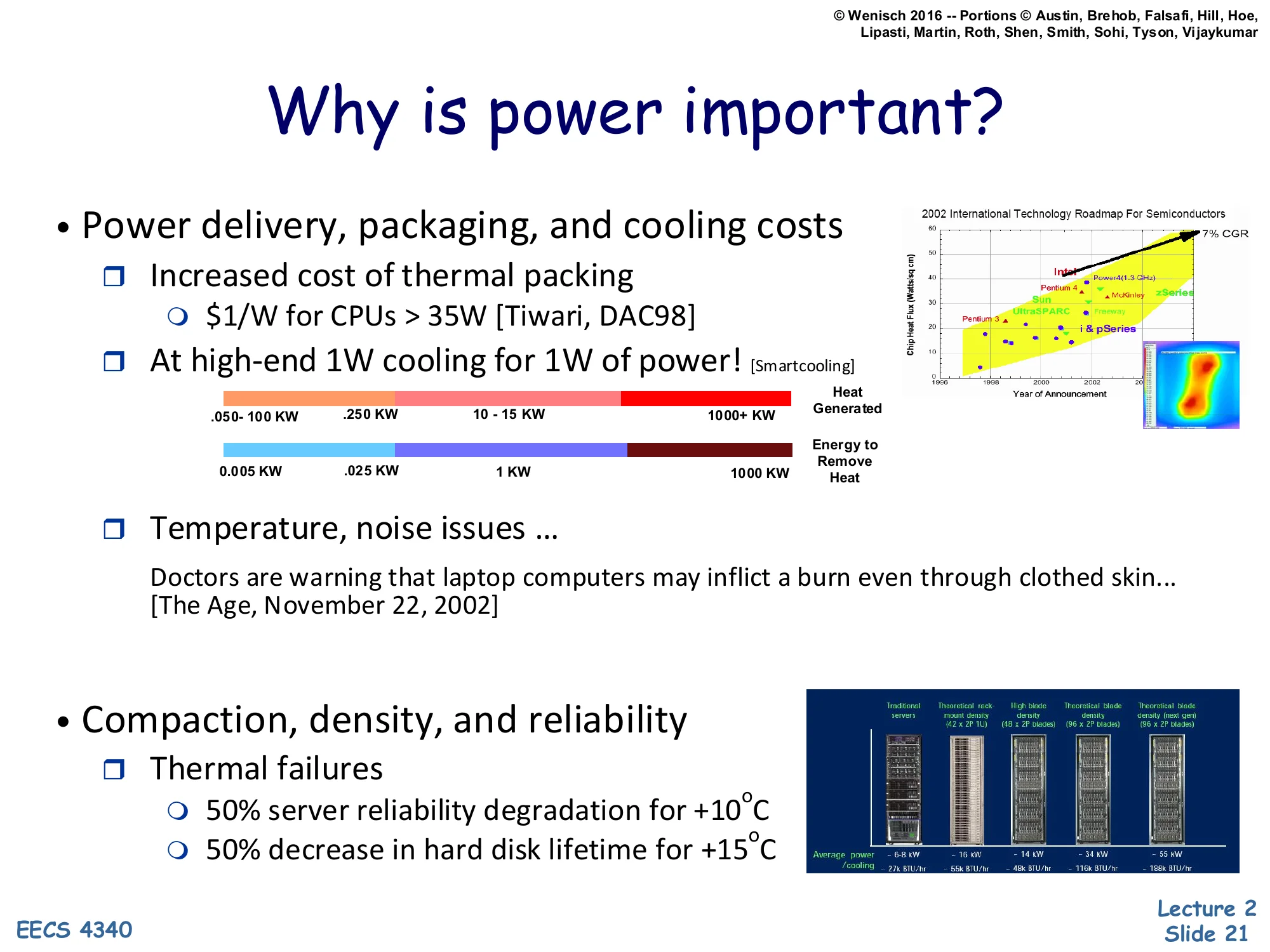
- Power delivery, packaging, and cooling costs
- Increased cost of thermal packaging
- $1/W for CPUs > 35W [Tiwari, DAC98]
- At high-end 1W for cooling for 1W of power! [Smartcooling]
- (Color bar: .050–100 KW … 250 KW … 10–15 KW … 1000+ KW; ITRS-style chart.)
- Increased cost of thermal packaging
- Temperature, noise issues …
- Doctors are warning that laptop computers may inflict a burn even through clothed skin… [The Age, November 22, 2002]
- Compaction, density, and reliability
- Thermal failures
- 50% server reliability degradation for +10°C
- 50% decrease in hard disk lifetime for +15°C
- Thermal failures
Even when total energy is acceptable, peak power is constrained by physical realities. Thermal packaging costs roughly $1 per watt for CPUs over 35 W (Tiwari, DAC ‘98), and at the top end the cooling system can consume as much power as the chip it’s cooling — 1 W of fans and chillers per 1 W of computation. The colored bar shows the wide spread of expected facility-level power over time, from tens of kilowatts up into the megawatt range as projected by the ITRS roadmap.
Power also creates secondary problems. Hot laptops literally injured users — the Age article from 2002 reports skin burns through clothing. Cooling fans add acoustic noise. And reliability degrades exponentially with temperature: every 10 °C above spec roughly halves server reliability, and every 15 °C roughly halves disk lifetime (Arrhenius behavior). So an unconstrained-power design might satisfy energy budgets while still being unshippable because it can’t meet packaging, acoustic, or reliability requirements. Peak watts are a hard ceiling, not just a soft preference.
Power: A first-class data center constraint
Show slide text
Power: A first-class data center constraint
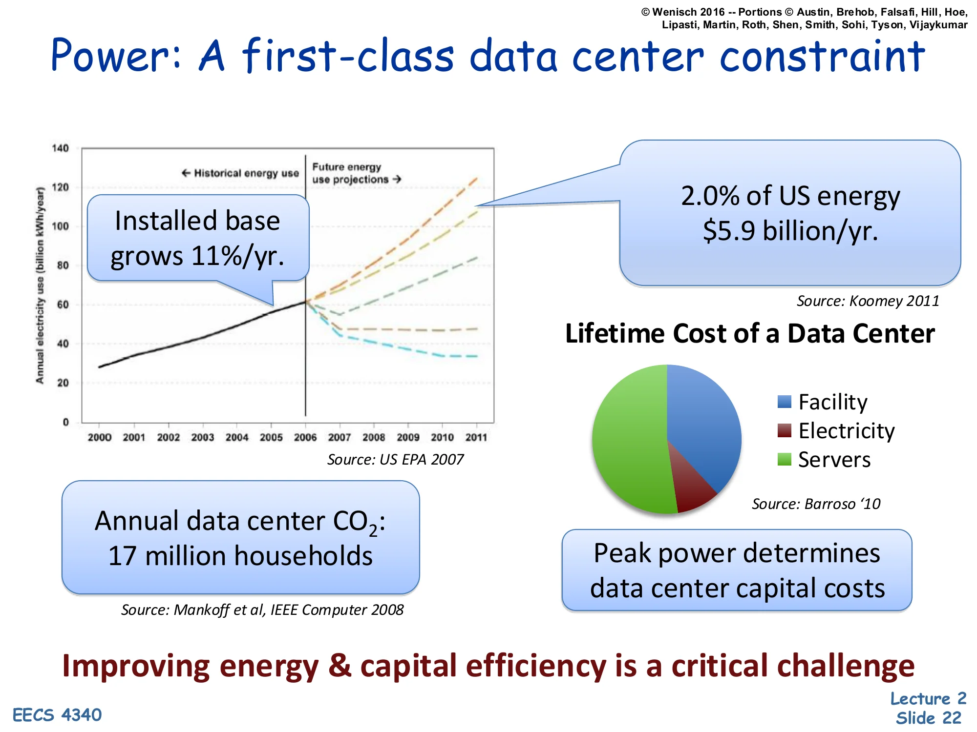
- Installed base grows 11%/yr.
- 2.0% of US energy, $5.9 billion/yr. [Source: Koomey 2011]
- Annual data center CO2: 17 million households [Source: Mankoff et al, IEEE Computer 2008]
- Lifetime Cost of a Data Center: Facility, Electricity, Servers (pie chart) [Source: Barroso ‘10]
- Peak power determines data center capital costs
Improving energy & capital efficiency is a critical challenge
By the early 2010s, datacenters consumed about 2% of US electricity — roughly $5.9 billion per year (Koomey 2011) — and the installed base grew about 11% annually. Annual datacenter CO₂ emissions matched roughly 17 million US households (Mankoff et al., IEEE Computer 2008). The pie chart on the right (Barroso 2010) breaks down the lifetime cost of a datacenter into facility (the building, power distribution, cooling), electricity, and servers; electricity and facility together typically dominate, especially since facility capital costs are themselves driven by peak power, not average.
That last point is the punchline of the slide: peak power determines capital costs because the building’s UPS, generator, transformer, and chiller capacity are all sized for the worst-case simultaneous power draw. A datacenter built for 10 MW peak costs roughly twice as much in facility capital as one built for 5 MW peak, regardless of average utilization. So squeezing peak watts out of the workload pays back in two places — lower electricity bill and lower buildout cost — making power-aware architecture economically central, not just environmentally desirable.
Server power breakdown
Show slide text
Server power breakdown
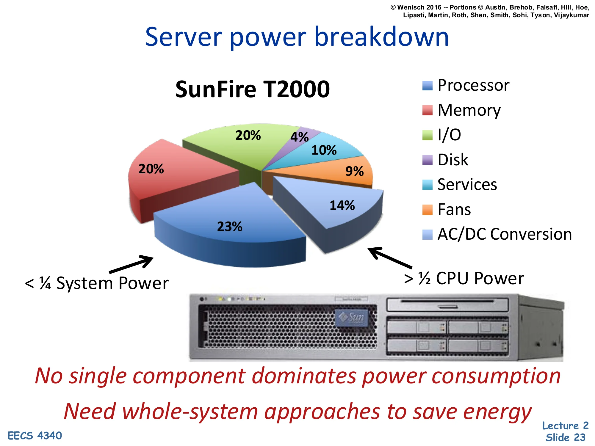
SunFire T2000 (pie chart):
-
Processor: 23%
-
Memory: 14%
-
I/O: 9%
-
Disk: 10%
-
Services: 4%
-
Fans: 20%
-
AC/DC Conversion: 20%
-
< 1/4 System Power (CPU)
-
1/2 CPU Power (other components combined)
No single component dominates power consumption. Need whole-system approaches to save energy.
The SunFire T2000 breakdown is the canonical “power is everywhere” data point. The processor accounts for only 23% of system power — less than a quarter — while memory takes 14%, disks 10%, I/O 9%, fans 20%, and AC/DC power conversion another 20%. The non-CPU components together (>50%) outweigh the CPU itself.
The lesson is that you cannot solve datacenter power by attacking the CPU alone. Even if you cut CPU power in half, total server power drops only ~12%. Fans and power-supply conversion losses are surprisingly large — modern designs attack these directly with variable-speed fans and 80-PLUS-rated supplies. Memory power scales with DIMM count and rank organization, which architects can influence. Disk power has shifted dramatically since this chart was made (rotational drives → SSDs change the curve). The general principle survives: power optimization must be a whole-system effort. Single-component focus produces diminishing returns once you’ve trimmed the obvious peaks.
What uses power in a chip

How CMOS Transistors Work
Show slide text
How CMOS Transistors Work
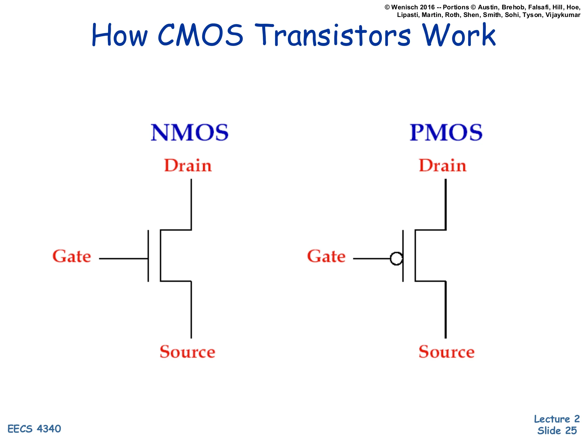
NMOS schematic: Drain (top), Gate (left, no bubble), Source (bottom).
PMOS schematic: Drain (top), Gate (left, with inversion bubble), Source (bottom).
CMOS — Complementary Metal-Oxide-Semiconductor — uses two transistor flavors. NMOS (n-channel) conducts when its gate voltage is high, pulling its drain toward whatever its source is connected to (typically ground). PMOS (p-channel) is the complement: it conducts when its gate is low, typically pulling its drain toward Vdd. The little circle (“bubble”) on the PMOS gate symbol marks this inversion convention.
In a CMOS gate the two flavors are paired so that exactly one of them conducts at a time in steady state — pull-up (PMOS network) toward Vdd when output should be high, pull-down (NMOS network) toward ground when output should be low. This complementary structure is what makes CMOS dramatically more energy-efficient than older NMOS-only logic: in steady state, no static current flows from Vdd to ground because one of the two networks is always off. Power is consumed only during the brief switching transition, which is the central insight that motivates the rest of the lecture’s power discussion.
MOS Transistors are Switches
Show slide text
MOS Transistors are Switches
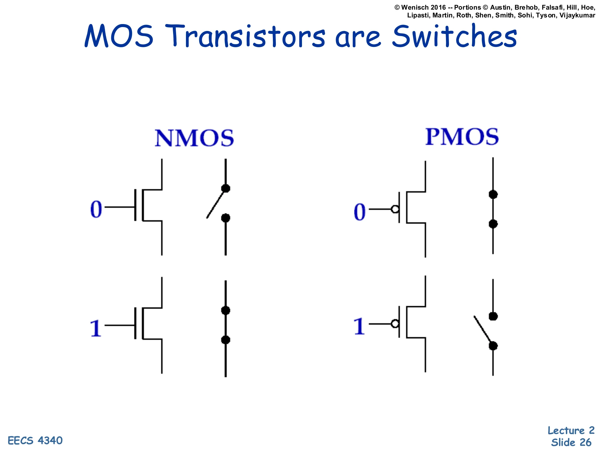
NMOS:
- Gate = 0: switch open (off)
- Gate = 1: switch closed (on)
PMOS:
- Gate = 0: switch closed (on)
- Gate = 1: switch open (off)
For the level of analysis used in this course, you can model CMOS transistors as ideal voltage-controlled switches. NMOS: gate high closes the switch (drain-to-source path conducts), gate low opens it. PMOS: the opposite — gate low closes the switch, gate high opens it. The schematic on the right of each pair literally redraws the transistor as an open or closed switch.
This abstraction lets you build logic gates by composing NMOS pull-down networks (in series for AND, in parallel for OR) with PMOS pull-up networks (the duals: parallel for AND output, series for OR output). The transistor-as-switch view is also the right starting point for thinking about power: the only times current flows through a CMOS gate are (a) while the switch is in transition (capacitive charging — dynamic power) and (b) leakage when the switch is supposedly off but isn’t truly — static power. Real transistors deviate from ideal switches in ways that drive the rest of the lecture: finite switching time, finite off-state resistance, threshold voltage variability.
Basic Logic Gates
Show slide text
Basic Logic Gates
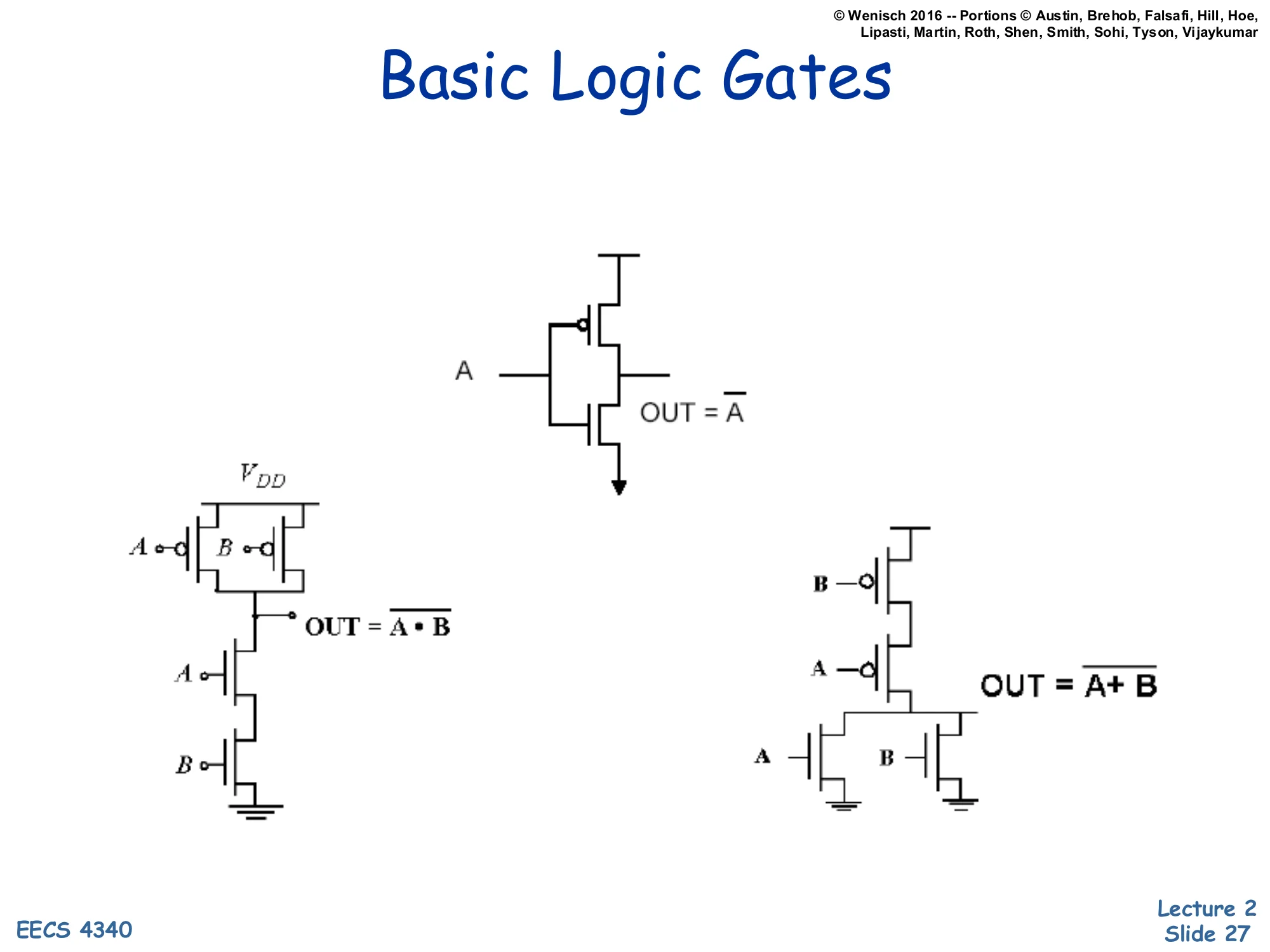
Inverter (NOT): single PMOS on top, single NMOS on bottom; A → OUT = A.
NAND: two PMOS in parallel (pull-up), two NMOS in series (pull-down); inputs A, B → OUT = A⋅B.
NOR: two PMOS in series (pull-up), two NMOS in parallel (pull-down); inputs A, B → OUT = A+B.
Three foundational CMOS gates demonstrate the dual-network design rule. The inverter (top) is the simplest: one PMOS connected to Vdd, one NMOS connected to ground, gates tied together. When input A is low, PMOS closes and NMOS opens — output pulled to Vdd (high). When A is high, the opposite — output pulled to ground (low). Hence OUT=A.
NAND (bottom-left) puts two PMOS in parallel on the pull-up side and two NMOS in series on the pull-down side. Output is low only when both A and B are high (both NMOS conducting); for any other input the output is pulled high by at least one PMOS. So OUT=A⋅B.
NOR (bottom-right) is the dual: two PMOS in series pull-up, two NMOS in parallel pull-down. Output is high only when both inputs are low. So OUT=A+B. The pattern — series-on-one-side, parallel-on-the-other, with PMOS and NMOS networks structurally dual — extends to arbitrary CMOS gates and is the foundation for both static logic design and the sizing decisions that determine switching speed.
Power: The Basics
Show slide text
Power: The Basics
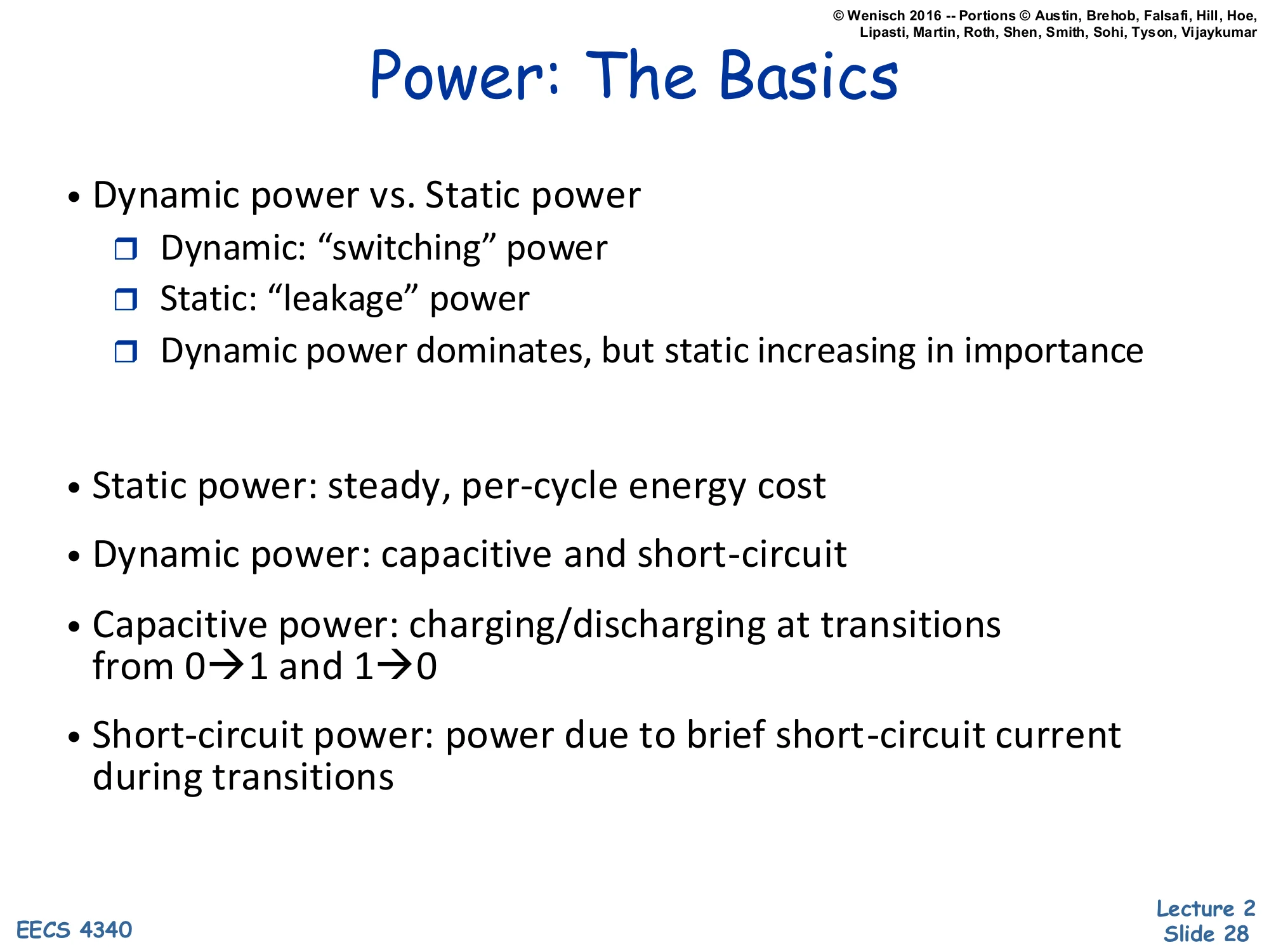
- Dynamic power vs. Static power
- Dynamic: “switching” power
- Static: “leakage” power
- Dynamic power dominates, but static increasing in importance
- Static power: steady, per-cycle energy cost
- Dynamic power: capacitive and short-circuit
- Capacitive power: charging/discharging at transitions from 0→1 and 1→0
- Short-circuit power: power due to brief short-circuit current during transitions
CMOS chips dissipate power in two regimes. Dynamic power scales with how often nodes toggle and with the voltage they swing; it is the cost of doing computation. Static (leakage) power flows whenever the chip is on, regardless of activity, because real transistors are not perfect switches. Historically dynamic power dominated, but as feature sizes shrank into deep sub-micron, leakage grew because the threshold voltage Vt had to drop to keep Vdd scaling viable, and subthreshold conduction grows exponentially as Vt drops.
Within dynamic power there are two sub-components. Capacitive switching power is the energy needed to charge a wire’s load capacitance from 0 to Vdd (or discharge it back) every time a node transitions; this is the term that the next slide’s 21CV2Af formula captures. Short-circuit power is the very brief NMOS-and-PMOS-both-conducting current spike during a transition, when the input voltage is between the two threshold voltages and both networks momentarily conduct simultaneously. Short-circuit power is usually a small fraction of dynamic power but grows when input slopes are slow.
Dynamic (Capacitive) Power Dissipation
Show slide text
Dynamic (Capacitive) Power Dissipation
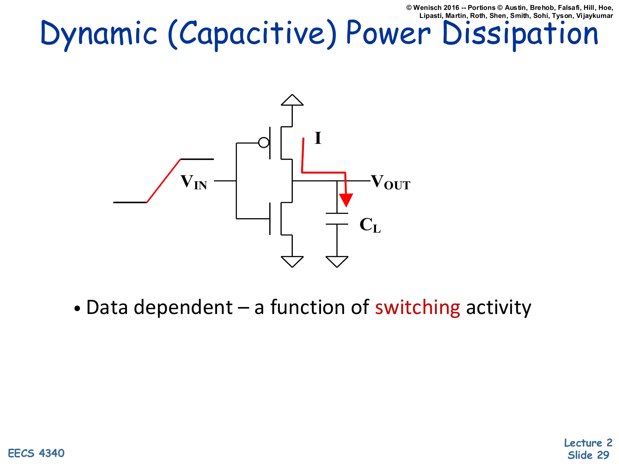
Schematic: CMOS inverter with VIN rising on left, current I flowing through PMOS to charge load capacitor CL at VOUT.
- Data dependent — a function of switching activity
The schematic shows a CMOS inverter at the moment its input rises from low to high. Before the rising edge, output was high — so the load capacitor CL at VOUT was charged to Vdd. As VIN rises, the PMOS turns off and the NMOS turns on, pulling VOUT down toward ground. The current I marked on the schematic flows from the capacitor through the NMOS to ground, draining stored charge Q=CLVdd.
On the next falling input edge the situation reverses: PMOS turns on, current flows from Vdd through PMOS into CL, recharging it. So every full 0→1→0 cycle moves total charge CLVdd through the chip, dissipating energy CLVdd2 — half stored in the capacitor and half lost as heat in the conducting transistor each transition. The bullet “Data dependent — a function of switching activity” is the key insight: nodes that don’t switch don’t burn dynamic power. The activity factor A (introduced on the next slide) is the average fraction of cycles a given node toggles, and it is the one term in the dynamic-power formula that microarchitects can attack with techniques like clock gating.
Capacitive Power dissipation
Show slide text
Capacitive Power dissipation
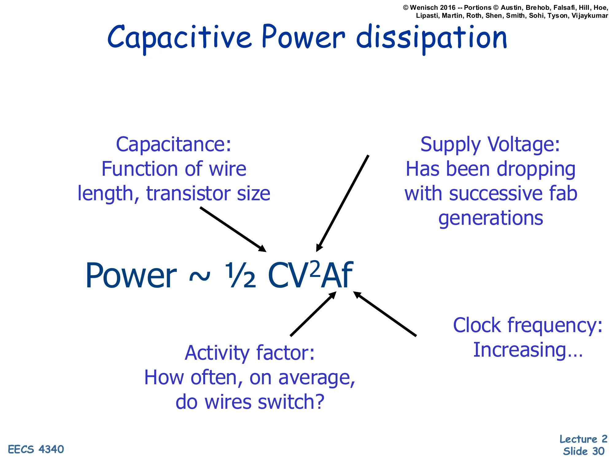
Power∼21CV2Af
- Capacitance: Function of wire length, transistor size
- Supply Voltage: Has been dropping with successive fab generations
- Activity factor: How often, on average, do wires switch?
- Clock frequency: Increasing…
The capacitive switching power equation P∼21CV2Af is the single most important formula in CMOS power analysis. Each factor is a knob with different tradeoffs.
Capacitance (C): total switched capacitance, dominated by interconnect (wire) capacitance and gate/diffusion capacitance. Scaling shrinks devices but lengthens average wire load relative to gate delay, so C has not dropped as fast as feature size. Lowered by smaller transistors and shorter wires.
Supply voltage (V): appears squared, so reductions are leveraged. Has historically dropped each fab generation (5 V → 3.3 V → 1.8 V → ~1 V) but is now near a floor set by transistor reliability and noise margins.
Activity factor (A): average fraction of cycles a given node switches. Microarchitectural — clock gating, data gating, operand isolation all target this term.
Clock frequency (f): linear factor. Historically increased with each generation, but plateaued in the 2000s as power exceeded packaging limits.
The formula is why DVFS (introduced two slides later) is so effective: lowering V together with f scales power roughly cubically in voltage.
Lowering Dynamic Power
Show slide text
Lowering Dynamic Power
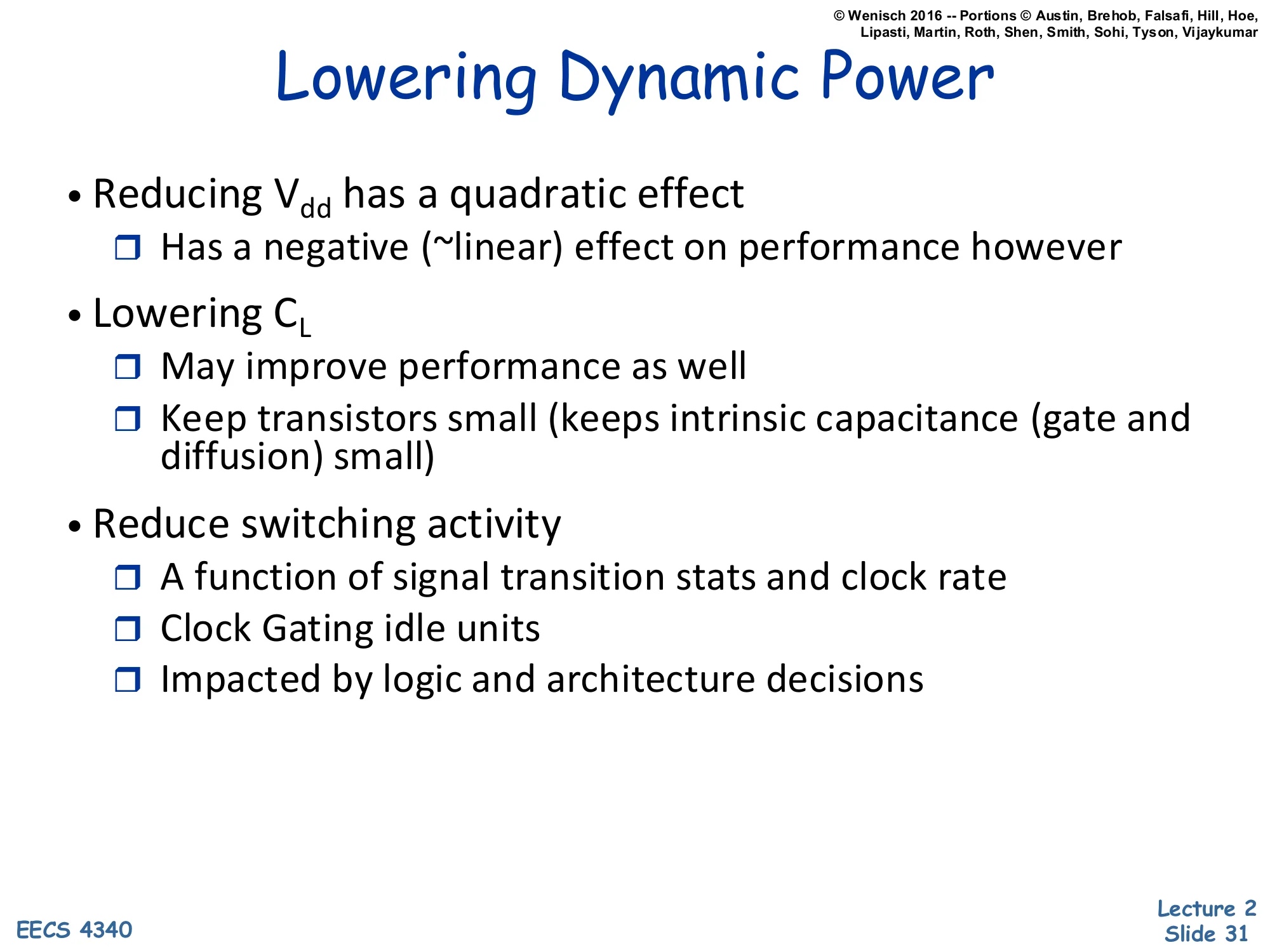
- Reducing Vdd has a quadratic effect
- Has a negative (~linear) effect on performance however
- Lowering CL
- May improve performance as well
- Keep transistors small (keeps intrinsic capacitance (gate and diffusion) small)
- Reduce switching activity
- A function of signal transition stats and clock rate
- Clock Gating idle units
- Impacted by logic and architecture decisions
Working term-by-term through P∼21CV2Af, this slide lists the levers a designer can pull to cut dynamic power. The voltage term is highest leverage because it appears squared — a 10% Vdd reduction yields a 19% power reduction (for the same f and A). But lowering Vdd also slows transistors roughly linearly, so it costs frequency unless you accept the slower clock; this is exactly the DVFS tradeoff.
Reducing capacitance helps both power and performance — smaller transistors have less gate and diffusion capacitance, charging/discharging faster, so this is a rare win-win. The constraint is drive strength: too small and the transistor can’t sink enough current to swing the next stage in one clock period.
Reducing activity factor A is where microarchitects spend most of their effort. Clock gating shuts off the clock to idle units (a register file’s read ports, an FPU when the pipeline holds only integer ops, an entire core when the OS schedules a sleep state). Data gating freezes input operands so combinational logic doesn’t switch when its result won’t be used. Architectural choices like banking, narrow-operand detection, and operand isolation all push the average activity factor down without touching V, C, or f.
DVFS: Dynamic Voltage/Frequency Scaling
Show slide text
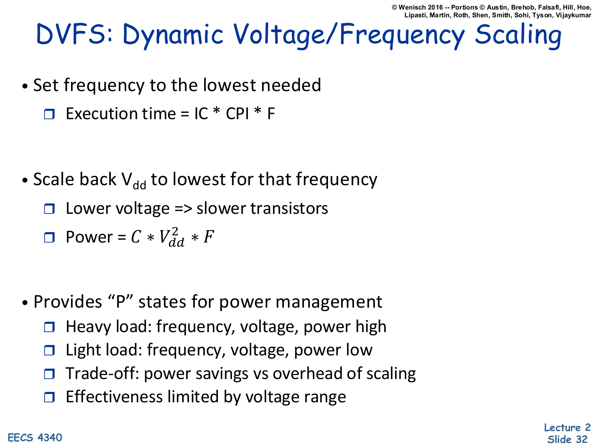
DVFS: Dynamic Voltage/Frequency Scaling
- Set frequency to the lowest needed
- Execution time = IC × CPI × F (i.e., IC × CPI / clock-rate)
- Scale back Vdd to lowest for that frequency
- Lower voltage ⇒ slower transistors
- Power = C⋅Vdd2⋅F
- Provides “P” states for power management
- Heavy load: frequency, voltage, power high
- Light load: frequency, voltage, power low
- Trade-off: power savings vs overhead of scaling
- Effectiveness limited by voltage range
DVFS is the textbook power-management technique. The recipe: pick the lowest clock frequency that still meets the workload’s deadline, then drop the supply voltage Vdd to the minimum value that supports that frequency reliably. Because power scales as CVdd2F and (when the voltage is near the gate-delay-limited regime) Vdd tracks F roughly linearly, total dynamic power scales roughly as V3 — a 10% slowdown can yield ~27% power savings.
The operating system exposes this through ACPI P-states: a discrete ladder of (voltage, frequency) operating points. Under heavy load the OS pushes the chip to the highest P-state (P0 — max V, max F, max power). Under light load it drops to lower P-states, trading throughput for power. Real systems pay an overhead each time they switch — the voltage regulator must slew, PLLs must relock — so changes can’t be too frequent.
DVFS effectiveness is bounded above by the maximum voltage allowed by reliability and bounded below by the minimum voltage at which transistors still switch correctly (typically 0.6–0.8 V for modern processes). Once you hit the lower wall, leakage starts dominating and further frequency cuts no longer save energy — sometimes called the “race to halt” regime where it pays to finish fast and sleep.
Static Power: Leakage Currents
Show slide text
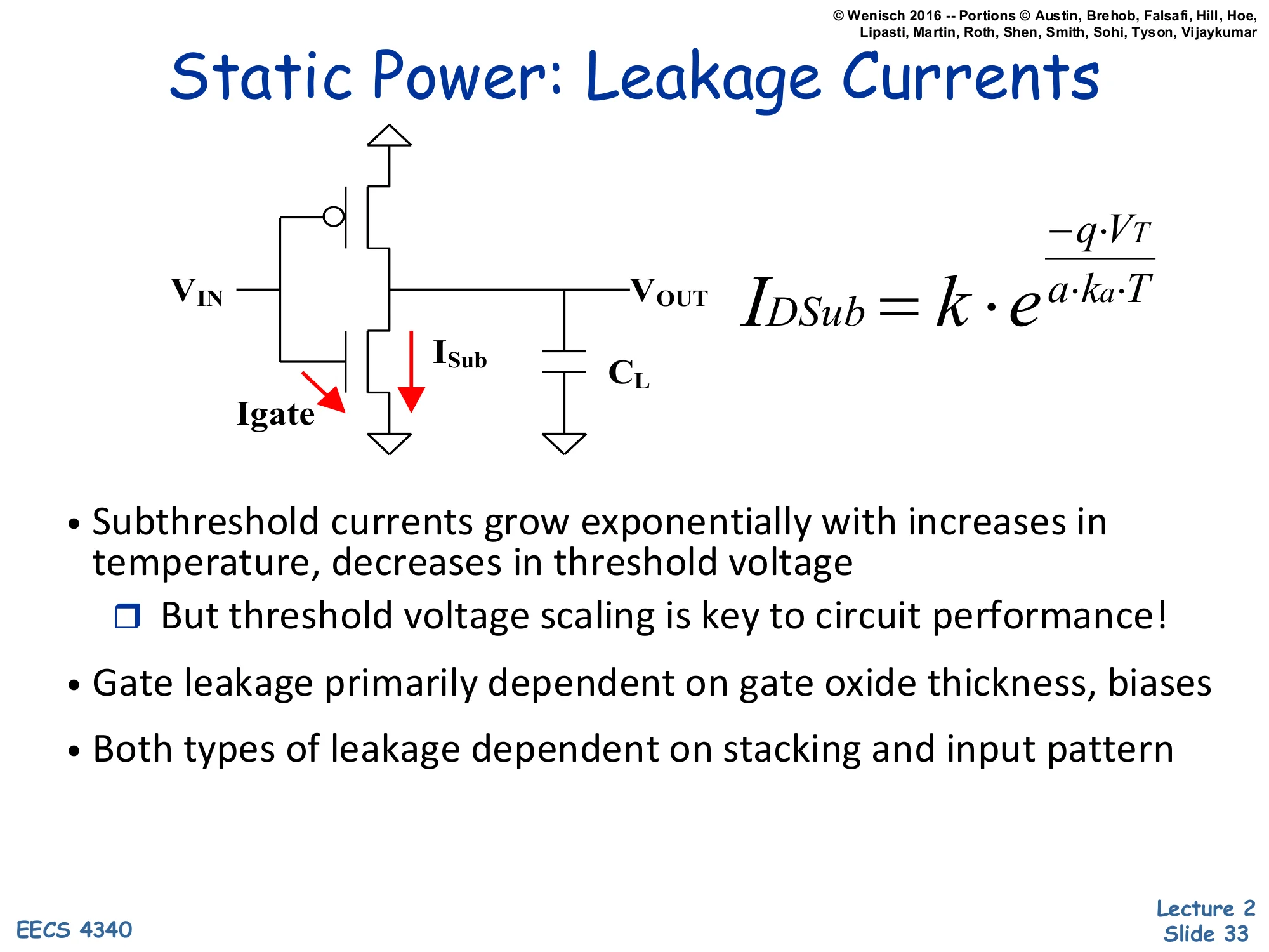
Static Power: Leakage Currents
Schematic: CMOS inverter with two leakage paths drawn in red — Igate through the gate oxide, and ISub through the off NMOS source-to-drain path; load capacitor CL at VOUT.
IDSub=k⋅ea⋅ka⋅T−q⋅VT
- Subthreshold currents grow exponentially with increases in temperature, decreases in threshold voltage
- But threshold voltage scaling is key to circuit performance!
- Gate leakage primarily dependent on gate oxide thickness, biases
- Both types of leakage dependent on stacking and input pattern
Real CMOS transistors leak current even when ostensibly off. The inverter schematic highlights two leakage components. ISub is subthreshold leakage: the off NMOS still conducts a small current from source to drain because the gate barrier is finite. The slide’s equation IDSub=k⋅e−qVT/(akaT) shows the dependence — exponential in threshold voltage VT (lower VT means more leakage) and exponential in temperature T (hotter chip means more leakage, which produces more heat, which can run away).
Igate is gate leakage: tunneling current through the thin gate oxide. As process generations shrank, gate oxides got thinner, and at sub-2 nm thickness electrons quantum-mechanically tunnel through. Gate leakage depends primarily on oxide thickness and bias.
The core tension: circuits get faster as VT drops (transistor turns on more strongly for a given Vdd), but leakage rises exponentially with that same VT drop. So fab generations push both directions — more performance and more static power per unit area. Both leakage types also depend on transistor stacking (multiple off transistors in series leak less than one) and input pattern (which transistors are biased on vs off), giving designers some architectural levers.
Lowering Static Power
Show slide text
Lowering Static Power
- Design-time Decisions
- Use fewer, smaller transistors — stack when possible to minimize contacts with Vdd/Gnd
- Multithreshold process technology (multiple oxides too!)
- Use “high-Vt” slow transistors whenever possible
- Dynamic Techniques
- Reverse-Body Bias (dynamically adjust threshold)
- Low-leakage sleep mode (maintain state), e.g. XScale
- Vdd-gating (Cut voltage/gnd connection to circuits)
- Zero-leakage sleep mode
- Lose state, overheads to enable/disable
- Reverse-Body Bias (dynamically adjust threshold)
Static (leakage) power can be attacked at design time and at runtime.
Design-time decisions. Use fewer transistors when possible — every transistor leaks. Stack transistors in series when feasible because two off transistors in series leak less than one alone (the body bias of the inner transistor self-reverses). Multi-Vt processes give the designer multiple transistor flavors: low-Vt fast transistors on the critical path, high-Vt slow but low-leakage transistors elsewhere. Multi-oxide processes provide a similar tradeoff for gate leakage.
Dynamic (runtime) techniques. Reverse-body bias temporarily raises Vt on idle blocks by biasing the substrate, dropping leakage by orders of magnitude while preserving stored state — Intel XScale used this for low-power sleep. Vdd-gating (also called power gating) cuts the supply connection entirely with a header or footer transistor, reducing leakage to essentially zero at the cost of losing all stored state in that block and paying a wakeup latency to re-establish voltage. Modern multicore SoCs apply Vdd-gating per core and sometimes per cache way, deeply sleeping unused units; the overhead is hundreds of cycles to enable and re-establish, so the OS only triggers it on long idle periods.
Combined Power-Performance Metrics
Show slide text
Combined Power-Performance Metrics
- Power-delay Product (PDP) = Pavg⋅t
- PDP is the average energy consumed per switching event
- Energy-delay Product (EDP) = PDP ⋅t
- Takes into account that one can trade increased delay for lower energy/operation
- Energy-delay2 Product (EDDP) = EDP ⋅t
- Why do we need so many formulas?!?
- We want a voltage-invariant efficiency metric! Why?
- Power ∼21CV2Af, Performance ∼f (and V)
Neither power nor performance alone tells the whole story; combined metrics let you compare designs that trade one for the other.
Power-delay product (PDP) = P⋅t. Since power times time is energy, PDP is energy per operation. Useful when energy efficiency is the goal (battery life, datacenter electricity bill).
Energy-delay product (EDP) = P⋅t2 = E⋅t. Multiplying by another t penalizes slow designs more heavily. Important when both energy and speed matter — you don’t want a design that saves a tiny bit of energy by running 10x slower.
Energy-delay2 product (ED²P) = P⋅t3=E⋅t2. Penalizes slowness even more heavily.
Why three metrics? The answer in the slide: we want a voltage-invariant efficiency metric. With DVFS, lowering voltage scales power as V2 (for fixed f) and slows performance as ∼1/V. The product P⋅tn is invariant under voltage scaling for the right exponent: ED²P is roughly voltage-invariant for typical DVFS curves, so it ranks designs by their intrinsic circuit/architecture quality rather than by where the operator chose to set the V/f knob. PDP and EDP are biased toward designs that happen to be tuned for low frequency.
E vs. EDP vs. ED²P
Show slide text
E vs. EDP vs. ED²P
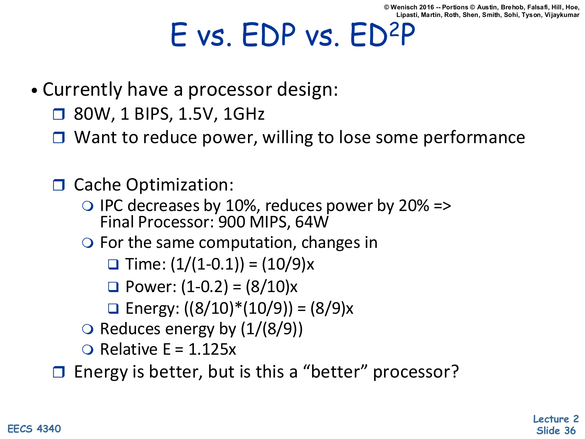
- Currently have a processor design:
- 80W, 1 BIPS, 1.5V, 1GHz
- Want to reduce power, willing to lose some performance
- Cache Optimization:
- IPC decreases by 10%, reduces power by 20% ⇒ Final Processor: 900 MIPS, 64W
- For the same computation, changes in
- Time: (1/(1−0.1))=(10/9)×
- Power: (1−0.2)=(8/10)×
- Energy: ((8/10)⋅(10/9))=(8/9)×
- Reduces energy by (1/(8/9))
- Relative E = 1.125×
- Energy is better, but is this a “better” processor?
A worked example shows how E, EDP, and ED²P can disagree. Baseline: 80 W, 1 BIPS (billion instructions per second), 1.5 V, 1 GHz. Proposed cache optimization: IPC drops 10% (so for the same computation, time grows by 10/9) but power drops 20% (so Pnew=0.8P). Final operating point: 900 MIPS at 64 W.
For the same computation, the changes are:
- Time: 10/9× longer (from the IPC drop)
- Power: 8/10× lower
- Energy = Power × Time = (8/10)(10/9)=8/9× — i.e., energy drops to about 89% of baseline, equivalently the baseline uses 9/8=1.125× as much energy as the optimized version.
So by the energy metric this looks like a clear win. But the slide ends with a leading question: “Is this a better processor?” The answer (revealed on the next slide) is that despite the energy improvement, EDP and ED²P tell a much less favorable story because the optimization gives up 10% of performance — and then there’s a comparison to plain DVFS, which can match the same 64 W with much smaller performance loss. The point is that picking the right metric depends on the design goal.
Not necessarily
Show slide text
Not necessarily
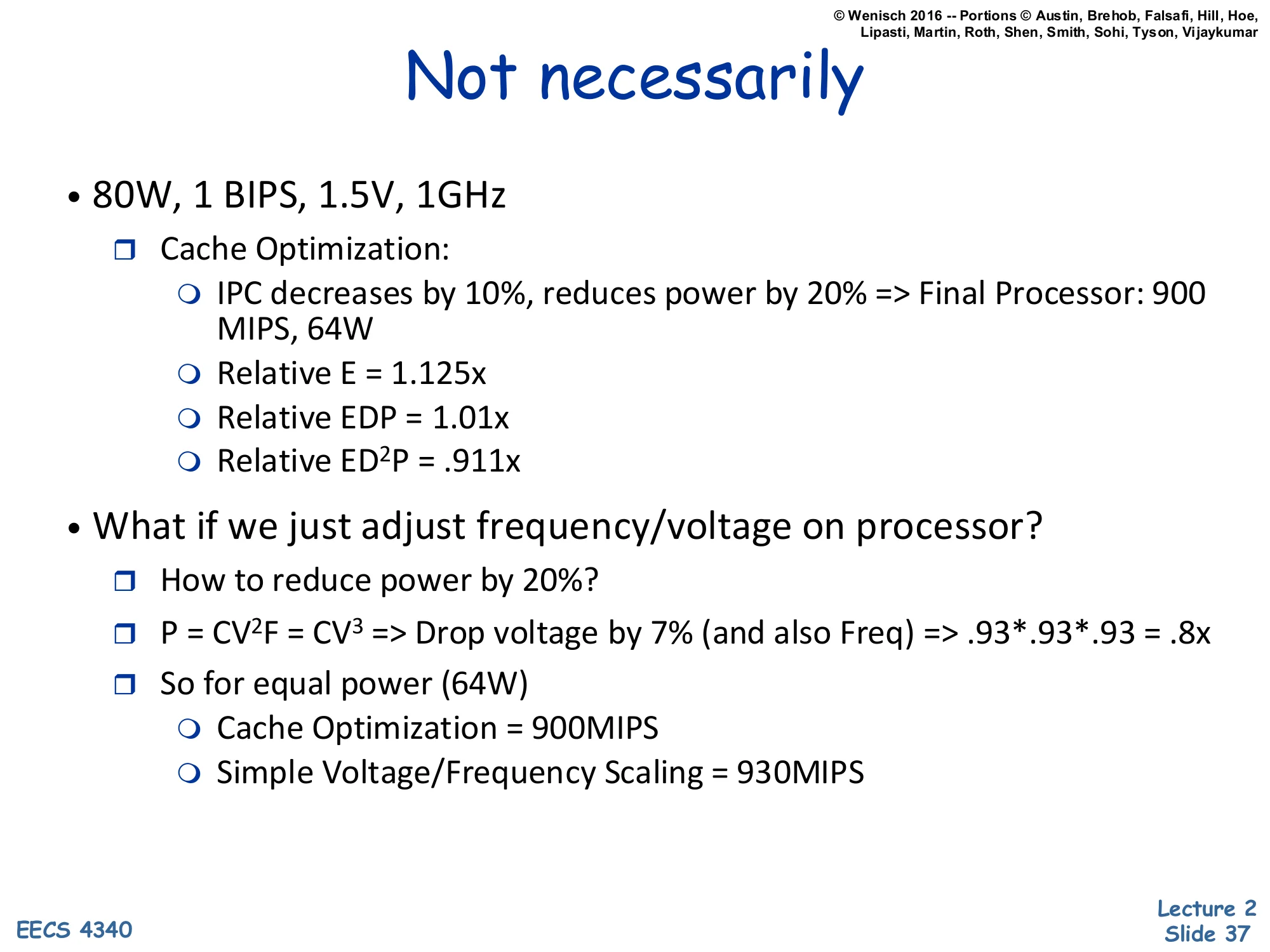
- 80W, 1 BIPS, 1.5V, 1GHz
- Cache Optimization:
- IPC decreases by 10%, reduces power by 20% ⇒ Final Processor: 900 MIPS, 64W
- Relative E = 1.125×
- Relative EDP = 1.01×
- Relative ED²P = .911×
- Cache Optimization:
- What if we just adjust frequency/voltage on processor?
- How to reduce power by 20%?
- P=CV2F=CV3⇒ Drop voltage by 7% (and also Freq) ⇒.93⋅.93⋅.93=.8×
- So for equal power (64 W)
- Cache Optimization = 900 MIPS
- Simple Voltage/Frequency Scaling = 930 MIPS
Continuing the example: by energy alone the cache optimization helps (relative E = 1.125× — baseline uses 12.5% more energy), and by EDP it’s roughly a wash (relative EDP = 1.01×). But by ED²P the cache optimization is worse (relative ED²P = 0.911× — baseline scores better) because the second factor of t penalizes the 10% slowdown heavily.
The more damning comparison is the alternative: simple DVFS on the original processor. Since dynamic power scales roughly as V3 when V∝f, dropping voltage (and frequency) by 7% gives 0.933≈0.8× — the same 20% power reduction as the cache optimization. But DVFS gives up only 7% of performance (linear in f), not 10%. At equal 64 W, the cache-optimized chip delivers 900 MIPS while DVFS delivers 930 MIPS. So the “clever” microarchitectural optimization is worse than just turning the V/f knob.
The broader lesson: any new architectural feature claiming power savings should be compared to the simplest possible alternative (DVFS), not to the original full-power baseline. ED²P, being approximately voltage-invariant, captures this comparison fairly; energy alone does not.
Class Problem (If Time)
Show slide text
Class Problem (If Time)
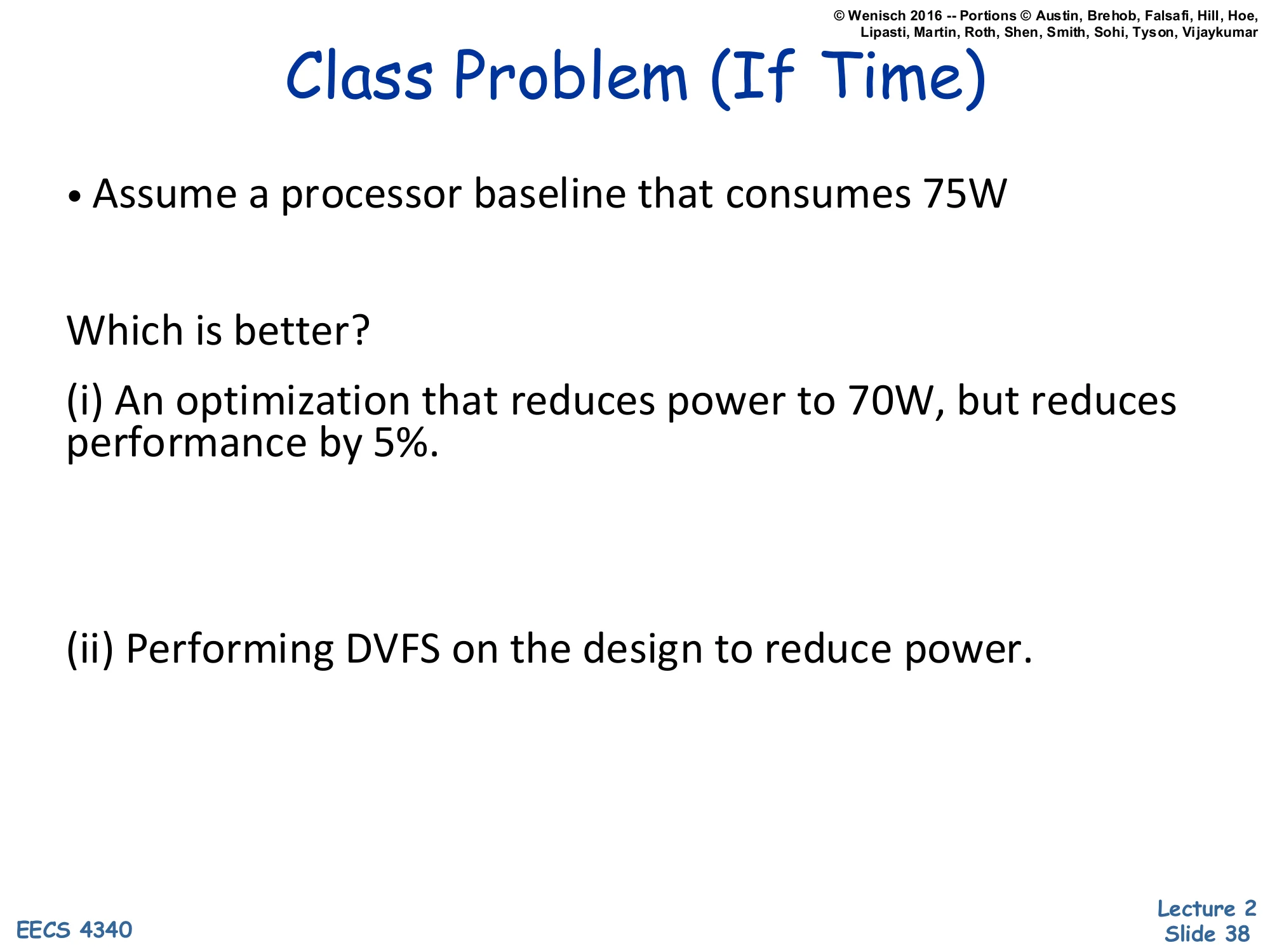
- Assume a processor baseline that consumes 75W
Which is better?
(i) An optimization that reduces power to 70W, but reduces performance by 5%.
(ii) Performing DVFS on the design to reduce power.
An in-class problem framed exactly like the previous slide’s example, asking students to apply the DVFS benchmark. Baseline: 75 W. Option (i) is a microarchitectural optimization that costs 5% performance for a power reduction from 75 W to 70 W (a 6.7% power cut). Option (ii) is plain DVFS on the same baseline, also reducing power. The question is: which is the better deal?
The right framing: at the same final power (or the same final performance), which option preserves more of the baseline’s capability? The next slide solves it. The expected approach is to compute how much performance DVFS gives up to reach the same 70 W, using the cubic-in-voltage relation, and compare to the 5% performance loss of option (i).
Class Problem (If Time) — Solution
Show slide text
Class Problem (If Time)
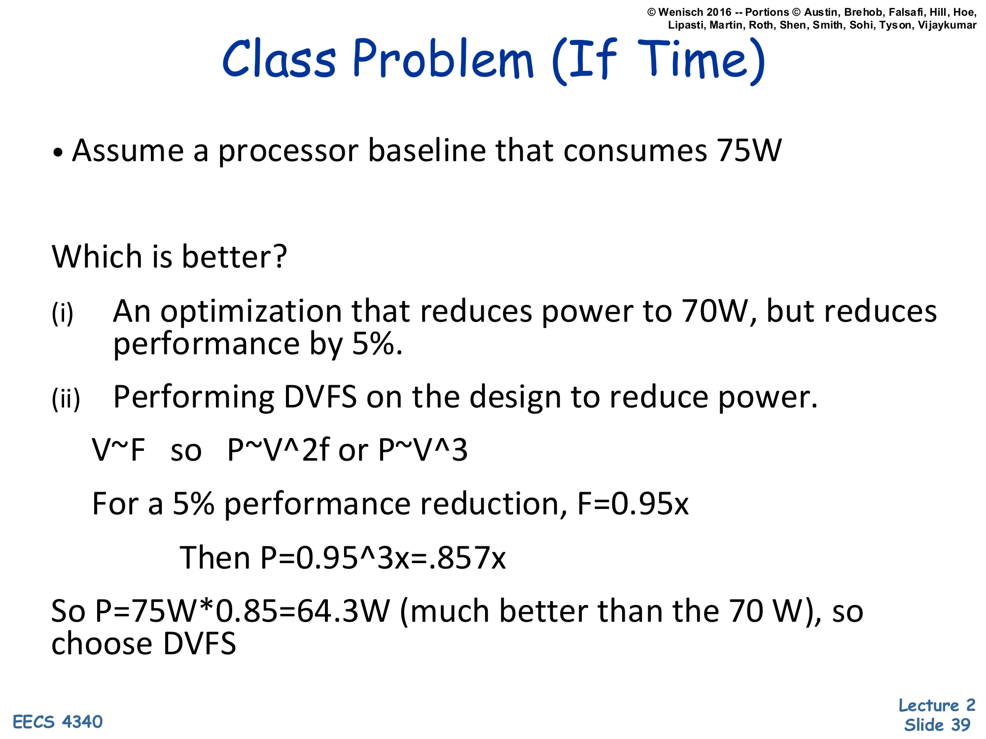
- Assume a processor baseline that consumes 75W
Which is better?
(i) An optimization that reduces power to 70W, but reduces performance by 5%.
(ii) Performing DVFS on the design to reduce power.
V∼F so P∼V2f or P∼V3
For a 5% performance reduction, F=0.95×
Then P=0.953×=.857×
So P=75W⋅0.85=64.3W (much better than the 70 W), so choose DVFS
The solution applies the cubic DVFS scaling. Assuming V∝F and P∝CV2f∼V3, accept the same 5% performance reduction as option (i): set F=0.95× baseline. Then power scales as 0.953≈0.857, so P=75⋅0.857≈64.3 W.
Compare: option (i) costs 5% performance and yields 70 W. Option (ii) costs the same 5% performance and yields only 64.3 W — significantly less power for identical performance loss. Therefore DVFS is the better choice; the proposed microarchitectural optimization is dominated.
This is the same lesson as the previous slide’s worked example: any new power-saving feature must beat plain V/f scaling, not just beat the original full-power baseline. DVFS is essentially “free” — no design effort, no extra silicon area — so it sets the floor that every clever microarchitectural power technique must exceed. Many published power optimizations fail this test, which is why ED²P (approximately voltage-invariant) is the preferred metric for fair comparison: it would have flagged option (i) as worse without needing to construct the explicit DVFS counterfactual.
Readings
Show slide text
Readings
For today:
- H & P Chapter 1
- H & P Appendix A
For next class:
- H & P Chapter C.1–C.4
Announcements

Show slide text
Announcements
Labs start this Wednesday
- Please bring your computer
- Involve graded assignments
- Attendance is required and graded
Project #1
- Will be released today (26-Jan-26)
- Due 4-Feb-26
- More details in the lab