L11 · Advanced Branch Prediction

L11 · Advanced Branch Prediction

Topic: branch-prediction · 52 pages

EECS 4340 Lecture 11 — Advanced Branch Prediction

Slide 1

Show slide text

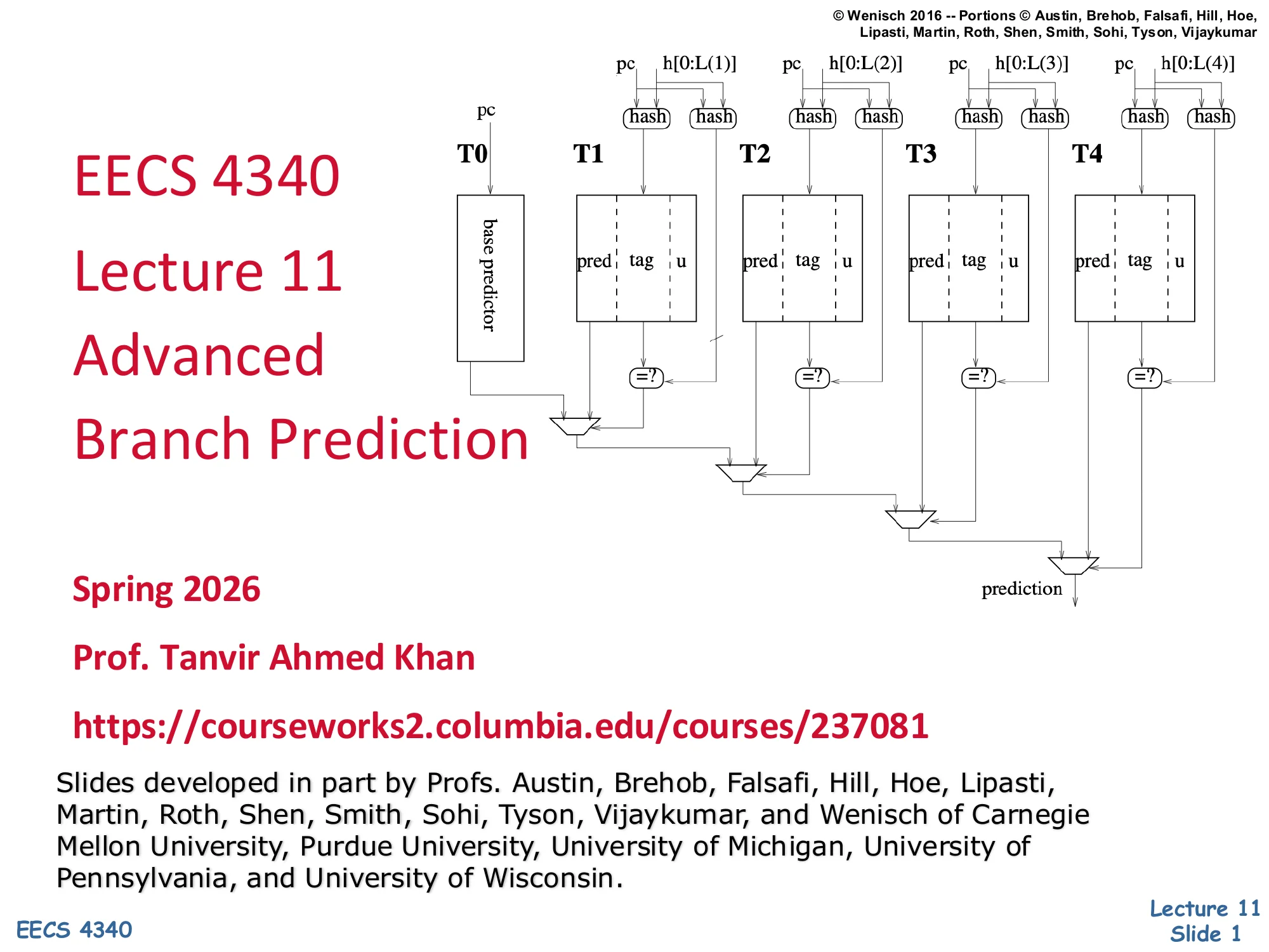
EECS 4340 — Lecture 11 — Advanced Branch Prediction

Spring 2026

Prof. Tanvir Ahmed Khan

https://courseworks2.columbia.edu/courses/237081

Slides developed in part by Profs. Austin, Brehob, Falsafi, Hill, Hoe, Lipasti, Martin, Roth, Shen, Smith, Sohi, Tyson, Vijaykumar, and Wenisch of Carnegie Mellon University, Purdue University, University of Michigan, University of Pennsylvania, and University of Wisconsin.

Cover diagram previews the TAGE multi-table tagged geometric history-length predictor: a base predictor T0 plus four tagged tables T1–T4 indexed by hashes of the PC and exponentially longer history h[0:L(i)].

Announcements

Slide 2

Show slide text

Announcements

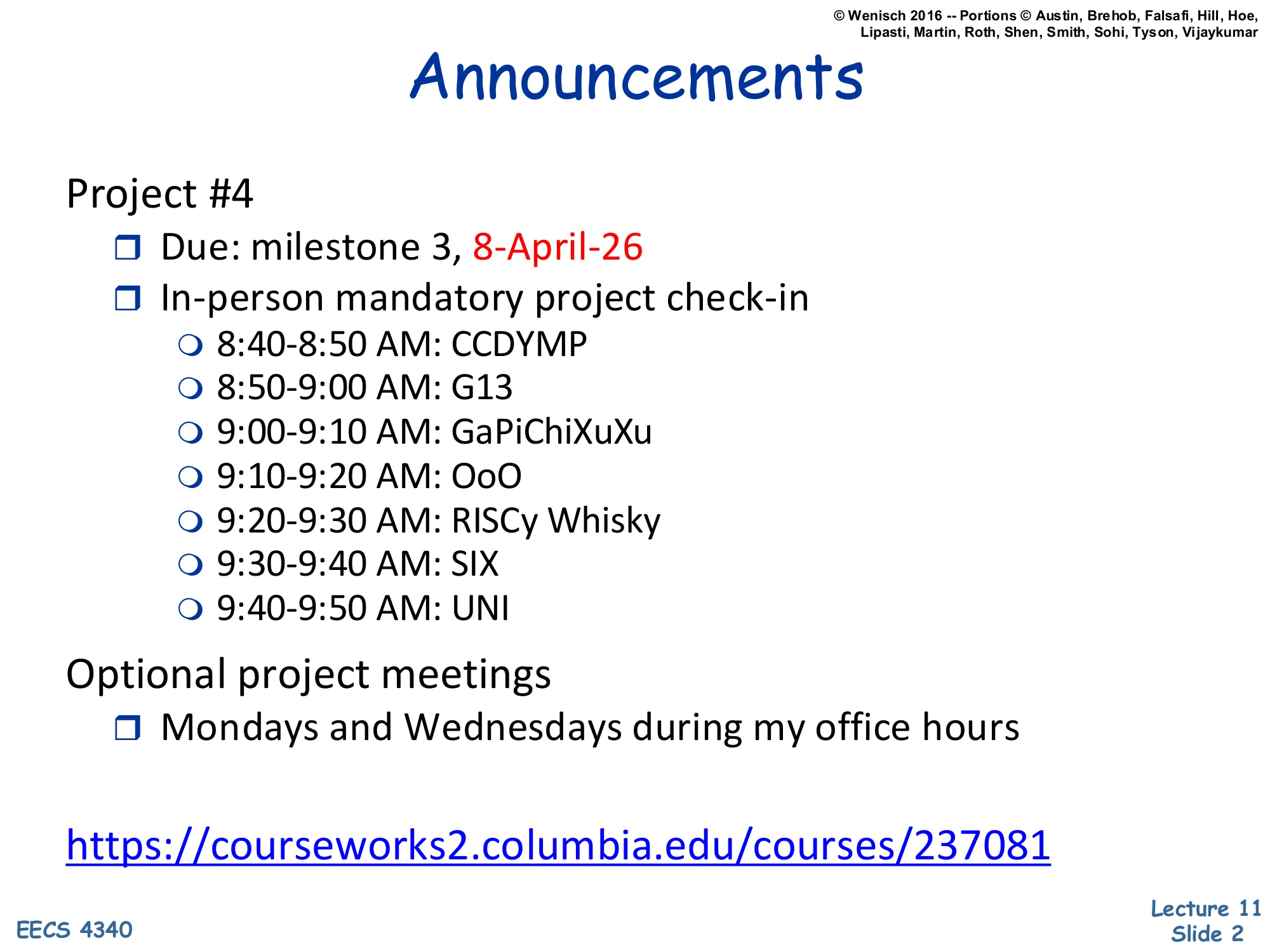
Project #4

• Due: milestone 3, 8-April-26
• In-person mandatory project check-in
  • 8:40–8:50 AM: CCDYMP
  • 8:50–9:00 AM: G13
  • 9:00–9:10 AM: GaPiChiXuXu
  • 9:10–9:20 AM: OoO
  • 9:20–9:30 AM: RISCy Whisky
  • 9:30–9:40 AM: SIX
  • 9:40–9:50 AM: UNI

Optional project meetings

• Mondays and Wednesdays during my office hours

https://courseworks2.columbia.edu/courses/237081

Readings

Slide 3

Show slide text

Readings

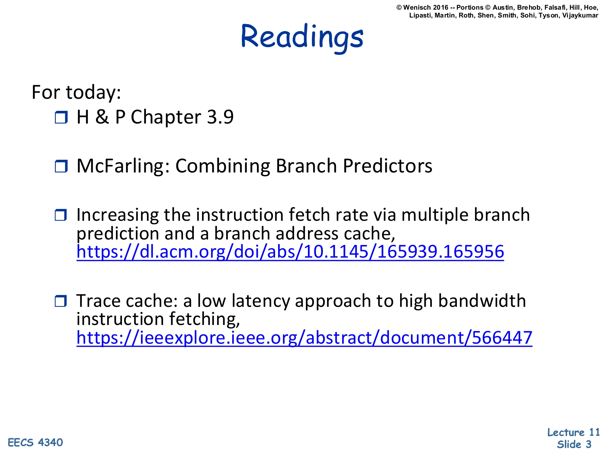
For today:

• H & P Chapter 3.9
• McFarling: Combining Branch Predictors
• Increasing the instruction fetch rate via multiple branch prediction and a branch address cache, https://dl.acm.org/doi/abs/10.1145/165939.165956
• Trace cache: a low latency approach to high bandwidth instruction fetching, https://ieeexplore.ieee.org/abstract/document/566447

The reading list pairs the textbook treatment of dynamic branch prediction (H&P 3.9) with three classic papers that ground the rest of the lecture. McFarling’s “Combining Branch Predictors” introduces the gshare hash and the tournament/hybrid predictor that picks between a per-PC bimodal counter and a global-history scheme. Yeh, Marr & Patt’s “Increasing the instruction fetch rate via multiple branch prediction and a branch address cache” shows how to predict more than one branch per cycle so a wide front end can keep up with an 8-issue back end. Rotenberg, Bennett & Smith’s “Trace cache” paper proposes a fetch structure that stores dynamic instruction sequences (traces) instead of static cache lines, sidestepping the alignment and collapsing problems caused by taken branches inside a fetch group. Together these readings span the two major dimensions of advanced front-end design: getting the prediction right (accuracy) and then keeping the pipeline fed when the prediction says “taken” (bandwidth).

Recap: Branch Prediction

Slide 4

Show slide text

Recap: Branch Prediction

Flow Path Model of CPU

Slide 5

Show slide text

Flow Path Model of CPU

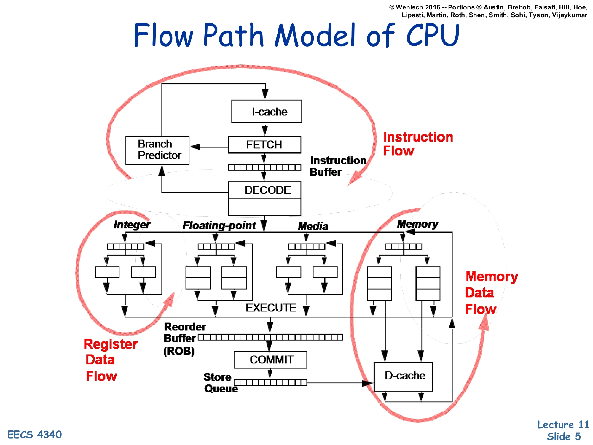
The pipeline diagram highlights three concurrent flows:

• Instruction Flow — I-cache → FETCH → instruction buffer → DECODE, with a feedback edge from the Branch Predictor back into FETCH.
• Register Data Flow — DECODE → reservation stations for Integer / Floating-point / Media / Memory units → EXECUTE → Reorder Buffer (ROB) → COMMIT.
• Memory Data Flow — Memory unit → store queue → D-cache.

Shen & Lipasti’s “flow path” model partitions an out-of-order core into three loops to make it clear where branch prediction sits. The instruction flow loop is the front end: the branch predictor reads the current PC, predicts the next-PC, and steers the I-cache lookup; if the predictor is wrong the entire loop must be flushed. The register data flow handles RAW dependences through reservation stations and the reorder buffer, which also enforces in-order commit so mispredictions can squash speculative state cleanly. The memory data flow runs through the store queue and D-cache. Branch prediction matters because every cycle the front end has no prediction it stalls, and every misprediction wastes all the work performed by the register and memory loops on the wrong path. The remainder of the lecture zooms in on the two halves of the predictor box drawn here: target prediction (next-PC for any control transfer) and direction prediction (taken/not-taken for conditional branches).

Branch Prediction (static vs dynamic)

Slide 6

Show slide text

Branch Prediction

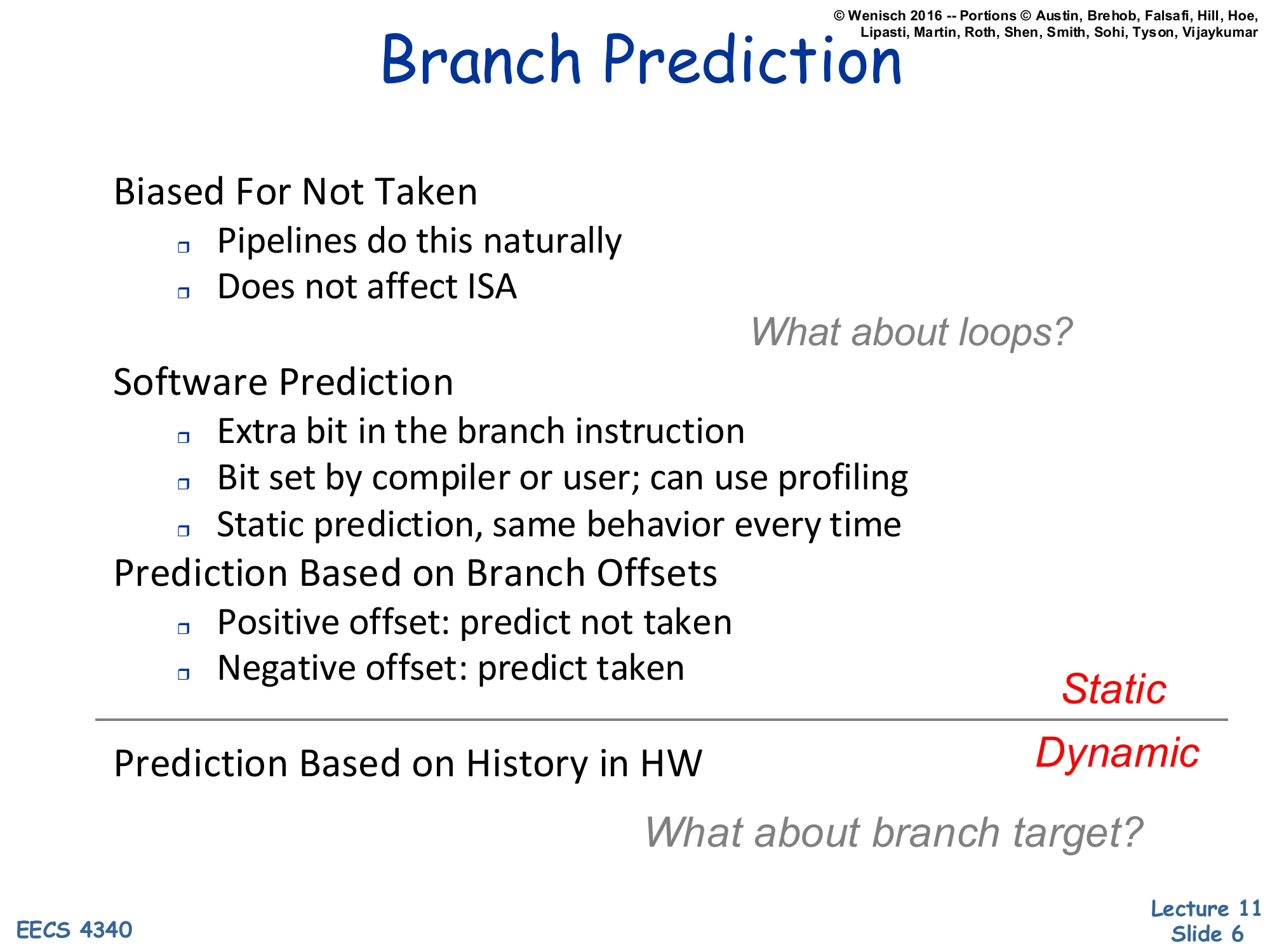
Static techniques:

• Biased For Not Taken
  • Pipelines do this naturally
  • Does not affect ISA — What about loops?
• Software Prediction
  • Extra bit in the branch instruction
  • Bit set by compiler or user; can use profiling
  • Static prediction, same behavior every time
• Prediction Based on Branch Offsets
  • Positive offset: predict not taken
  • Negative offset: predict taken

Dynamic techniques:

• Prediction Based on History in HW — What about branch target?

The slide separates static prediction (decision fixed at compile time) from dynamic prediction (decision based on runtime history in hardware). “Always not taken” is essentially free because the standard fetch pointer already speculates down the fall-through path; its weakness is loops, where the loop-back branch is taken almost every iteration. Software prediction encodes a hint bit in the branch instruction (set by the compiler or by profile-guided optimization) so the predictor knows the static bias without having to learn it. Backwards-taken/forwards-not-taken (BTFNT) exploits the observation that loop-back branches have negative offsets and forward branches typically guard rare cases. None of these schemes adapt to phase changes within a single execution. Dynamic branch prediction addresses that by tracking outcomes at runtime — and it has to solve two problems at once: predict the direction of conditional branches and predict the target of any control transfer (call, return, indirect jump, taken branch).

Dynamic Branch Prediction

Slide 7

Show slide text

Dynamic Branch Prediction

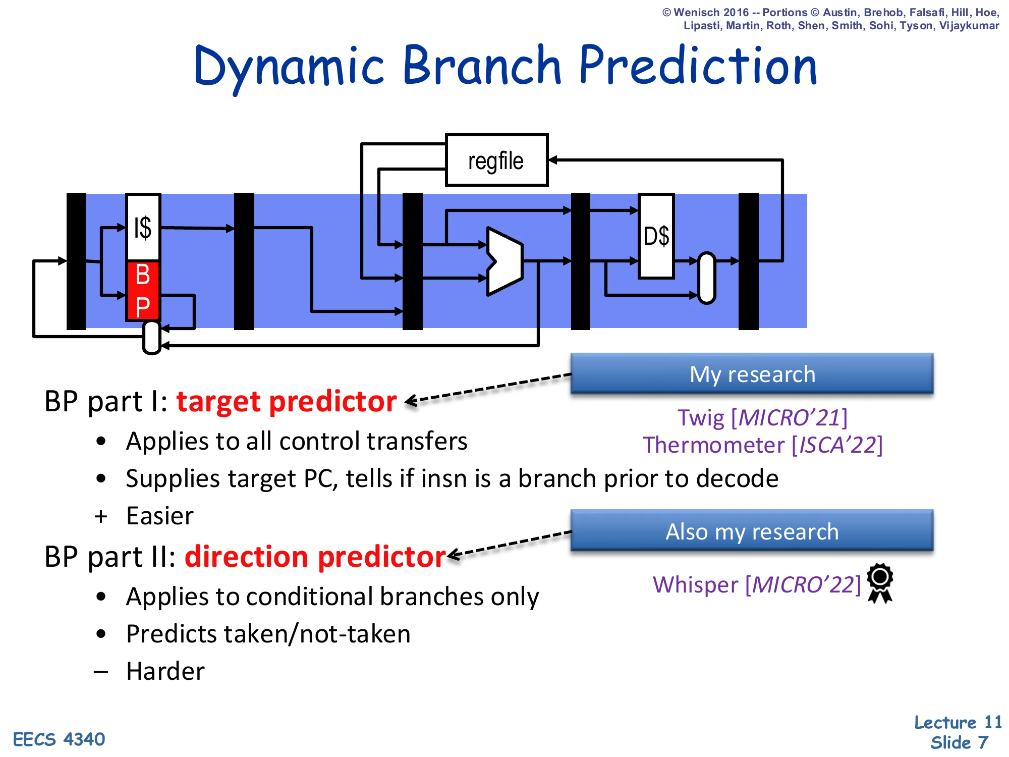
A pipeline diagram shows the BP block sitting next to the I$ in the fetch stage with a feedback loop back to the next-PC mux.

BP part I: target predictor

• Applies to all control transfers
• Supplies target PC, tells if insn is a branch prior to decode
• (+) Easier
• Recent research: Twig [MICRO’21], Thermometer [ISCA’22]

BP part II: direction predictor

• Applies to conditional branches only
• Predicts taken/not-taken
• (–) Harder
• Recent research: Whisper [MICRO’22]

Dynamic branch prediction is split into two cooperating predictors. The target predictor is queried for every fetch address and answers two questions: “is this instruction a control transfer?” and “if it is taken, where does it go?” Without this predictor the front end could not even tell that a branch existed until decode, by which time the next fetch cycle has already committed to PC+4. The direction predictor only matters for conditional branches and chooses between the fall-through path and the taken target. Direction prediction is harder because conditional branches are often weakly biased and depend on data that has not yet been computed, while indirect call and return targets are constrained by the program’s call structure. The professor flags two of his own research projects (Twig, Thermometer) on the target side and one (Whisper) on the direction side to motivate that this is still an active research area, not a solved problem.

Branch Target Buffer (BTB)

Slide 8

Show slide text

Branch Target Buffer

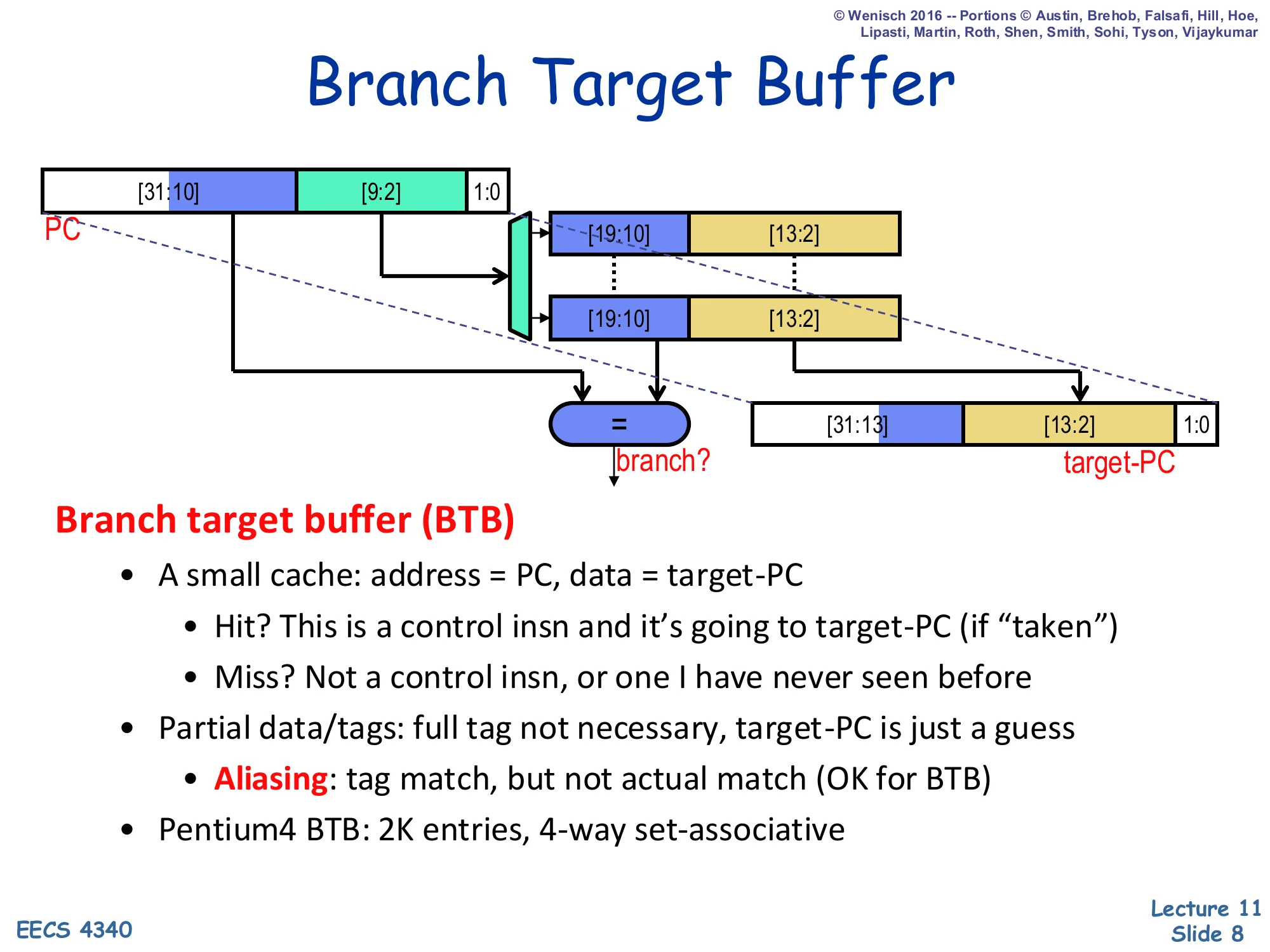
The diagram shows a 32-bit PC split into tag bits [31:10], index bits [9:2], and offset bits [1:0]. Index selects a BTB entry storing a tag [19:10] and a partial target [13:2]; an =? comparator decides hit/miss and the stored target [13:2] is concatenated with the upper PC bits to form target-PC.

Branch target buffer (BTB)

• A small cache: address = PC, data = target-PC
  • Hit? This is a control insn and it’s going to target-PC (if “taken”)
  • Miss? Not a control insn, or one I have never seen before
• Partial data/tags: full tag not necessary, target-PC is just a guess
  • Aliasing: tag match, but not actual match (OK for BTB)
• Pentium 4 BTB: 2K entries, 4-way set-associative

The branch target buffer is the hardware that answers the target-prediction question in one fetch cycle. It is a small cache indexed by the fetch PC; a hit means “this PC is a control transfer I have seen before, and last time it went to this target.” A miss means either the instruction is not a branch or the BTB has not learned about it yet, so the front end falls back to the sequential next-PC. Because the BTB only supplies a prediction, partial tags are fine: an aliasing match between two PCs that share the low-order tag bits costs at most one misprediction the first time the new branch executes — there is no correctness issue. The Pentium 4 example (2 K entries × 4 ways) is typical of mid-2000s designs; modern cores push BTBs into the tens of thousands of entries because instruction footprints have grown. The picture is also why the BTB is integrated with set associativity: associativity reduces destructive aliasing for branches that map to the same set.

Return Address Stack (RAS)

Slide 9

Show slide text

Return Address Stack (RAS)

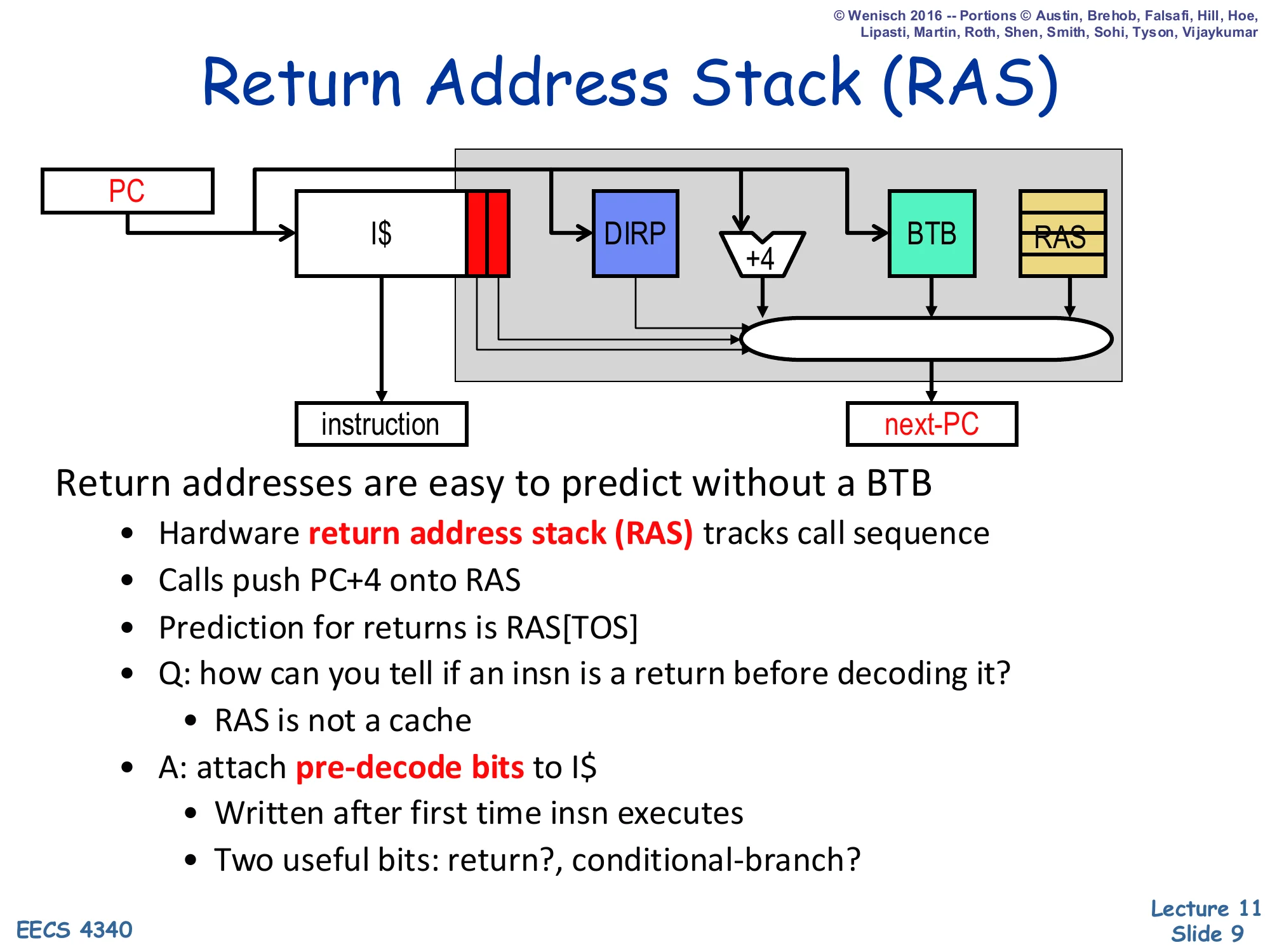
The fetch-stage diagram shows the PC fanning out to the I$, to the DIRP (direction predictor), to a +4 adder, to the BTB, and to the RAS, with the four candidate next-PCs muxed into next-PC. Pre-decode bits attached to the I-cache line tell the mux which source to pick.

Return addresses are easy to predict without a BTB

• Hardware return address stack (RAS) tracks call sequence
• Calls push PC+4 onto RAS
• Prediction for returns is RAS[TOS]
• Q: how can you tell if an insn is a return before decoding it?
  • RAS is not a cache
• A: attach pre-decode bits to I$
  • Written after first time insn executes
  • Two useful bits: return?, conditional-branch?

Returns are the worst-case input to a BTB because the same return instruction (the ret at the end of a callee) jumps to many different targets — one for each call site. A BTB indexed by the return PC would predict whichever caller called most recently. The return address stack solves this by mirroring the program’s call/return structure: every call pushes PC+4 (the address right after the call) onto a small hardware stack, and every return pops the top-of-stack as its predicted target. As long as the call/return discipline is balanced and the stack is deep enough, returns are predicted with near-100% accuracy. The remaining wrinkle is recognising a return before decode. Pre-decode bits, written into the I-cache the first time the instruction executes, mark each cache-line slot with two flags — is_return? and is_conditional? — so the front end can route the prediction through the RAS or the DIRP without waiting for a real decode.

Branch Direction Prediction

Slide 10

Show slide text

Branch Direction Prediction

Direction predictor (DIRP)

• Map conditional-branch PC to taken/not-taken (T/N) decision
• Seemingly innocuous, but quite difficult
• Individual conditional branches often unbiased or weakly biased
  • 90%+ one way or the other considered “biased”

The direction predictor (DIRP) is the second half of dynamic branch prediction. Its input is a conditional branch’s PC and its output is a single bit: taken or not-taken. The slide flags how surprisingly hard this is. A naive intuition is that branches are heavily skewed — and many indeed are — but “biased” in the literature means at least 90% one-way. The remaining ~50% of dynamic branches are weakly biased (somewhere between 60–90%) or essentially balanced, which is where every percentage point of additional accuracy comes from. Because mispredictions cost an entire pipeline-depth’s worth of wrongly fetched, dispatched, and partially executed instructions on a modern out-of-order core, even moving from 95% to 97% accuracy is a measurable IPC win. The next several slides build progressively more powerful DIRP designs, starting with a per-PC table of single bits and ending at TAGE.

Branch History Table (BHT)

Slide 11

Show slide text

Branch History Table (BHT)

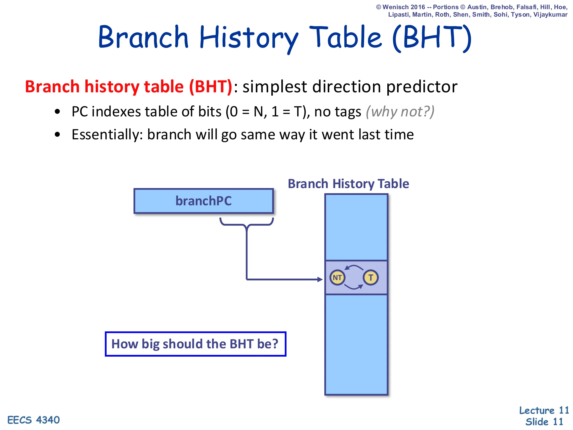
Branch history table (BHT): simplest direction predictor

• PC indexes table of bits (0 = N, 1 = T), no tags (why not?)
• Essentially: branch will go same way it went last time

A diagram shows branchPC indexing a column-shaped Branch History Table whose entry is a tiny 1-bit FSM with two states NT ↔ T.

How big should the BHT be?

A branch history table is the cheapest direction predictor: take the low-order PC bits, index a table of 1-bit counters, and predict the state of that bit (0 = not taken, 1 = taken). The slide deliberately notes “no tags (why not?)”. Like a BTB, the table only stores a prediction, so an aliasing collision between two branches that hash to the same row simply costs at most one misprediction; there is no correctness issue, and tags would double the storage cost. The implicit FSM behind each bit is trivial: predict the last outcome. This works fine on heavily biased branches but pathologically mispredicts loop-exit branches twice per loop nest — the very last iteration flips the bit, and the bit then mispredicts the first iteration of the next entry into the loop. The fix appears two slides later as the 2-bit saturating counter. Sizing the BHT is a textbook capacity-vs-collision trade-off: too small and unrelated branches alias; too large and you spend area on entries that are barely used.

Two-Bit Saturating Counters (2bc)

Slide 12

Show slide text

Two-Bit Saturating Counters (2bc)

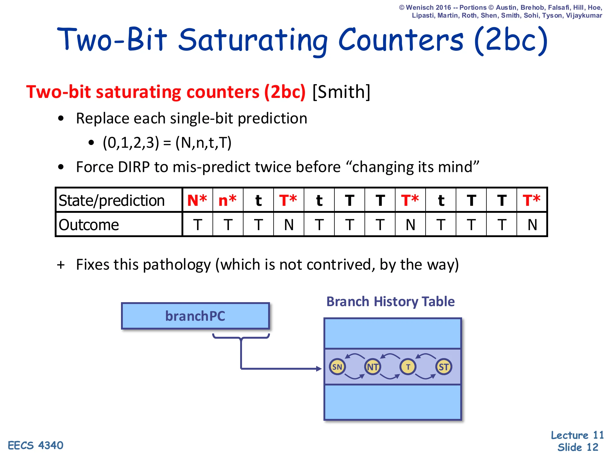
Two-bit saturating counters (2bc) [Smith]

• Replace each single-bit prediction
  • $(0,1,2,3) = (N, n, t, T)$ — strongly-not-taken, weakly-not-taken, weakly-taken, strongly-taken
• Force DIRP to mis-predict twice before “changing its mind”

State/prediction	N*	n*	t	T*	t	T	T	T*	t	T	T	T*
Outcome	T	T	T	N	T	T	T	N	T	T	T	N

• Fixes this pathology (which is not contrived, by the way)

The automaton has four states SN → NT → T → ST with arrows on each side showing taken/not-taken transitions.

The two-bit saturating counter, due to Jim Smith, replaces each 1-bit BHT entry with a 4-state FSM (SN, NT, T, ST). The high-order bit is the prediction; the low-order bit acts as hysteresis. To flip the prediction the counter has to be wrong twice in a row, which exactly matches the loop-exit pathology shown in the trace: a loop body that goes T,T,T,N over and over wastes only one misprediction (on the N) per loop entry, instead of two for the 1-bit predictor. The four-state automaton is also why bimodal predictors with 2bc hit ~85% accuracy on SPEC integer codes — they capture per-PC bias robustly without history. The lecture stresses that the pathology is “not contrived”: nearly every loop in real code looks like this, so the upgrade from 1-bit to 2-bit counters is essentially free (it doubles storage but reuses the same indexing logic) and is universally adopted in the BHT entries of every modern predictor as the base predictor.

Advanced Branch Prediction

Slide 13

Show slide text

Advanced Branch Prediction

Using More History: Correlated Predictor

Slide 14

Show slide text

Using More History: Correlated Predictor

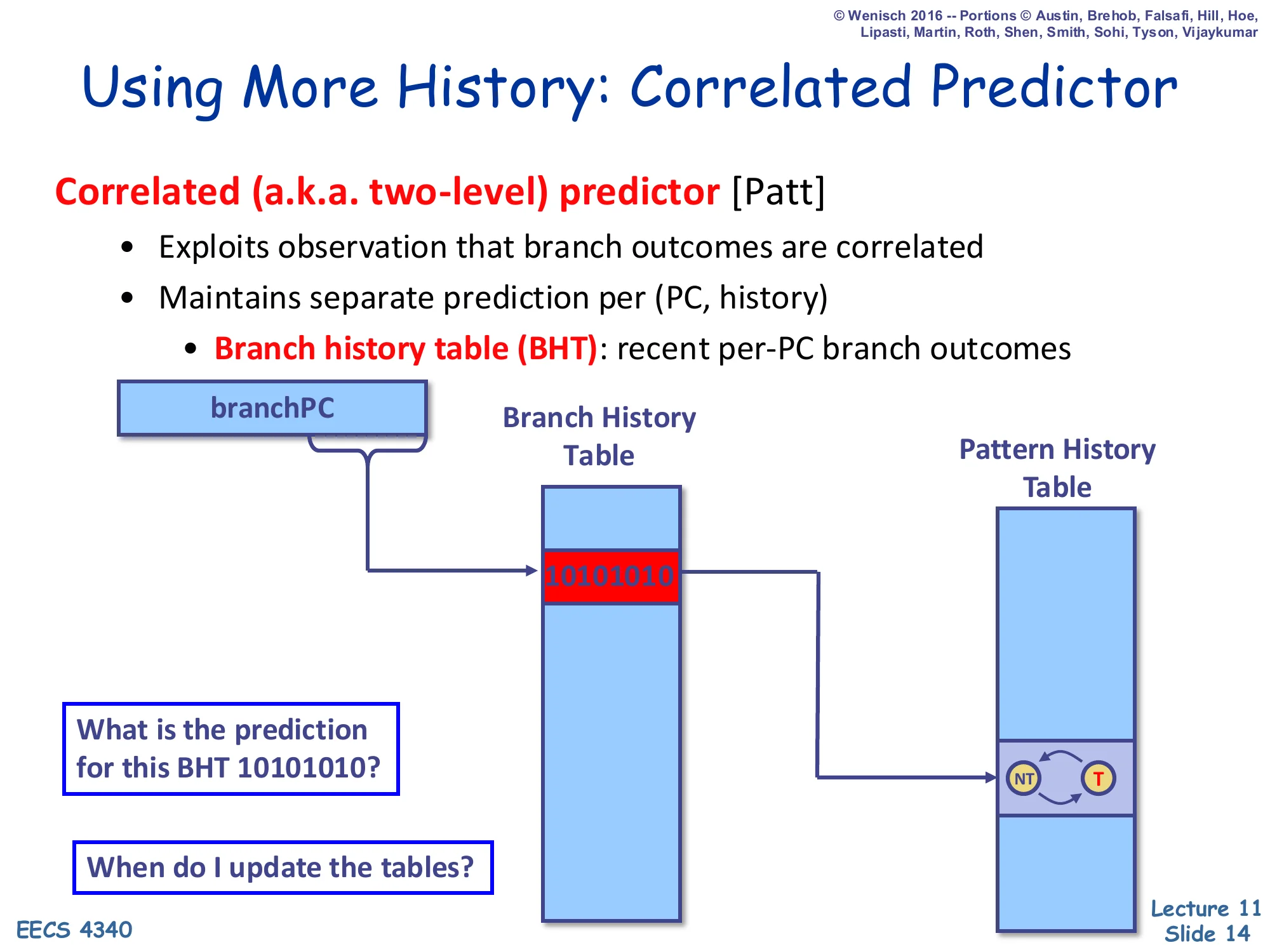
Correlated (a.k.a. two-level) predictor [Patt]

• Exploits observation that branch outcomes are correlated
• Maintains separate prediction per (PC, history)
  • Branch history table (BHT): recent per-PC branch outcomes

Diagram: branchPC indexes a per-PC Branch History Table; the row shown holds the bit-string 10101010, which then indexes a Pattern History Table whose entry is a 2-state NT ↔ T counter.

What is the prediction for this BHT 10101010?

When do I update the tables?

Yeh and Patt’s correlated (two-level) predictor recognises that a branch’s behaviour is often a function of recent branch history, not just of its own past outcomes. The first level is a branch history table — but here BHT means a small per-PC shift register that records the last k outcomes of that branch. The second level is a Pattern History Table (PHT) of 2-bit counters indexed jointly by the PC and that history. So a branch that flips between taken and not taken in the pattern 10101010… gets a separate counter for each history bit-string and can therefore predict each phase of the pattern correctly. The two design questions on the slide preview the next sequence of slides: the question “prediction for BHT 10101010?” leads into the worked example that traces convergence, and “when do I update?” foreshadows the speculative-update problem solved later by checkpointing the BHR on every prediction.

Correlated Predictor Example — Initial State

Slide 15

Show slide text

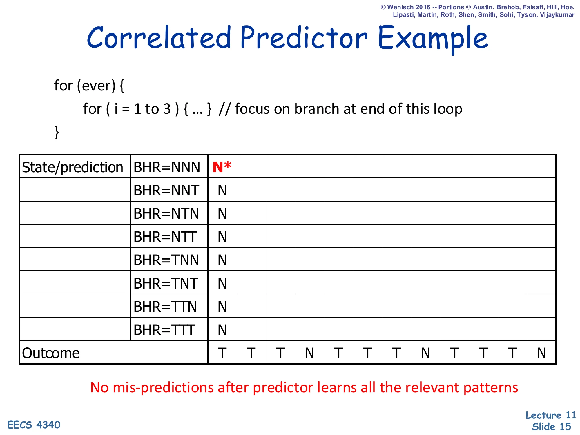
Correlated Predictor Example

for (ever) {
  for (i = 1 to 3) { ... }   // focus on branch at end of this loop
}

State/prediction
BHR=NNN	N*
BHR=NNT	N
BHR=NTN	N
BHR=NTT	N
BHR=TNN	N
BHR=TNT	N
BHR=TTN	N
BHR=TTT	N
Outcome	T	T	T	N	T	T	T	N	T	T	T	N

No mis-predictions after predictor learns all the relevant patterns

The example focuses on the inner-loop back-edge of a 3-iteration for loop wrapped inside an infinite outer loop. The branch outcome stream is therefore the periodic pattern T T T N, and a 3-bit branch history register (BHR) gives enough context to make every iteration distinguishable. At time 0 every PHT row is initialised to predict not-taken (N), the BHR is NNN, and the cell that will be consulted first is starred (N*). The bottom row spells out the next 12 outcomes the program will produce. The point of the slide is that even though the outcome stream is periodic, the (BHR, outcome) pairs that the predictor will see are not, because the BHR shifts in the most recent outcome each time. The next four slides walk one step at a time through the cells the predictor reads and updates, showing how the table converges to a state with zero mispredictions.

Correlated Predictor Example — Step 2

Slide 16

Show slide text

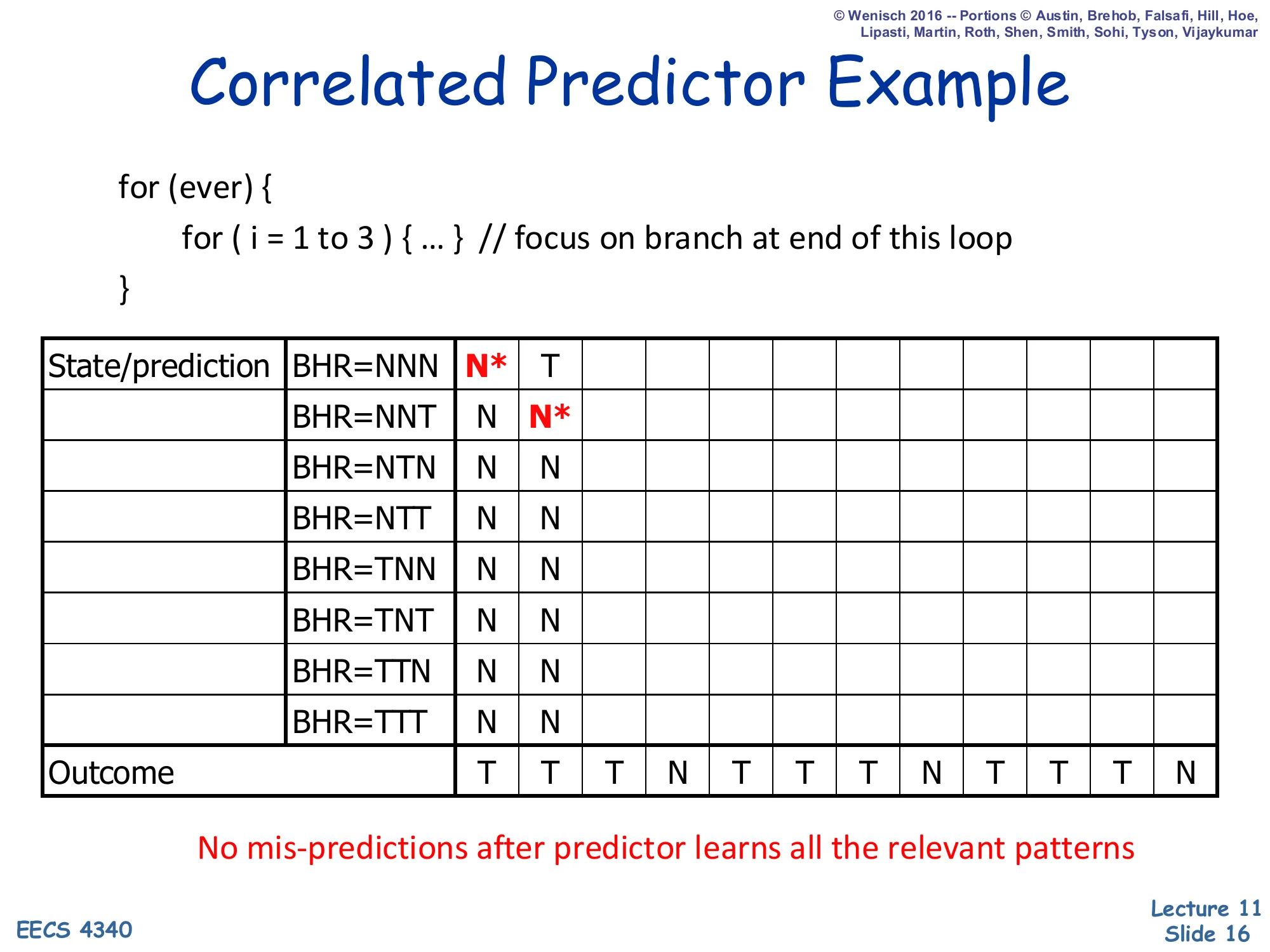
Correlated Predictor Example

for (ever) {
  for (i = 1 to 3) { ... }   // focus on branch at end of this loop
}

State/prediction
BHR=NNN	N*	T
BHR=NNT	N	N*
BHR=NTN	N	N
BHR=NTT	N	N
BHR=TNN	N	N
BHR=TNT	N	N
BHR=TTN	N	N
BHR=TTT	N	N
Outcome	T	T

No mis-predictions after predictor learns all the relevant patterns

Step 2: the first outcome was T, so the BHR shifts from NNN to NNT and the previous PHT entry is updated from N to T (the column-1 cell now reads T). The starred cell — the one being consulted now — is the row BHR=NNT, which still predicts N. The outcome is again T (we are inside the body of the inner loop), so this cell will also be updated to T in the next step. The animation makes the key point of correlation: the same dynamic branch instruction is making two different predictions in two consecutive cycles because the BHR distinguishes “first iteration of the inner loop” from “second iteration.” A simple bimodal BHT without history would have mixed all three iterations together and converged to predict T 75% of the time, mispredicting the loop-exit on every outer iteration.

Correlated Predictor Example — Step 3

Slide 17

Show slide text

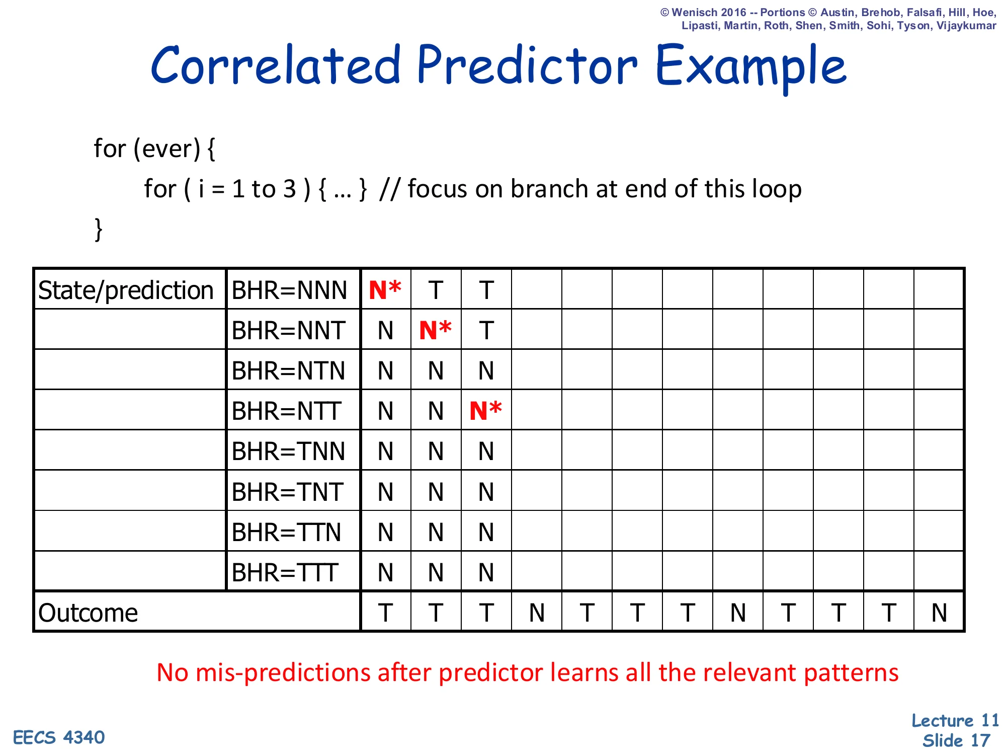
Correlated Predictor Example

for (ever) {
  for (i = 1 to 3) { ... }   // focus on branch at end of this loop
}

State/prediction
BHR=NNN	N*	T	T
BHR=NNT	N	N*	T
BHR=NTN	N	N	N
BHR=NTT	N	N	N*
BHR=TNN	N	N	N
BHR=TNT	N	N	N
BHR=TTN	N	N	N
BHR=TTT	N	N	N
Outcome	T	T	T

No mis-predictions after predictor learns all the relevant patterns

Step 3: the BHR is now NTT (oldest bit on the left). The starred cell — the active read — is the row BHR=NTT, which still holds the initial value N. The two cells that were active in steps 1 and 2 have been updated to T to reflect the two taken outcomes seen so far. The active cell will mispredict on this cycle (outcome will be T but prediction is N), then itself flip to T. After three iterations of taken outcomes the predictor has installed T in three different rows, one for each (history, branch) pair; the fourth iteration, where the loop exits, will install an N into row BHR=TTT. Notice that no two iterations of the inner loop ever consult the same PHT row, which is exactly the property that makes a correlated predictor strictly more powerful than a per-PC bimodal predictor for any periodic pattern shorter than the BHR.

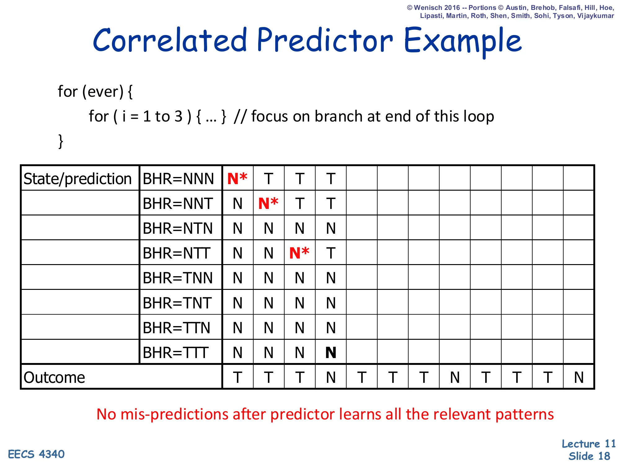
Correlated Predictor Example — Step 4

Slide 18

Show slide text

Correlated Predictor Example

for (ever) {
  for (i = 1 to 3) { ... }   // focus on branch at end of this loop
}

State/prediction
BHR=NNN	N*	T	T	T
BHR=NNT	N	N*	T	T
BHR=NTN	N	N	N	N
BHR=NTT	N	N	N*	T
BHR=TNN	N	N	N	N
BHR=TNT	N	N	N	N
BHR=TTN	N	N	N	N
BHR=TTT	N	N	N	N
Outcome	T	T	T	N

No mis-predictions after predictor learns all the relevant patterns

Step 4: the BHR is now TTT (three taken outcomes in a row). The active cell is row BHR=TTT, which currently predicts N. The actual outcome will be N as well, because this is the iteration that exits the inner loop — so this is a correct prediction even though the predictor has not yet “learned” anything about the pattern, by sheer luck of the initial state. The cell remains at N and the BHR shifts to TTN for the next prediction. After this point the predictor is in steady state: every (BHR, outcome) pair it will ever see has been written with the correct answer at least once, so unless the loop pattern changes, every subsequent prediction is correct. The slide’s highlighted bottom-right N is the lucky coincidence; the next slide shows that this cell is in fact stable forever afterward.

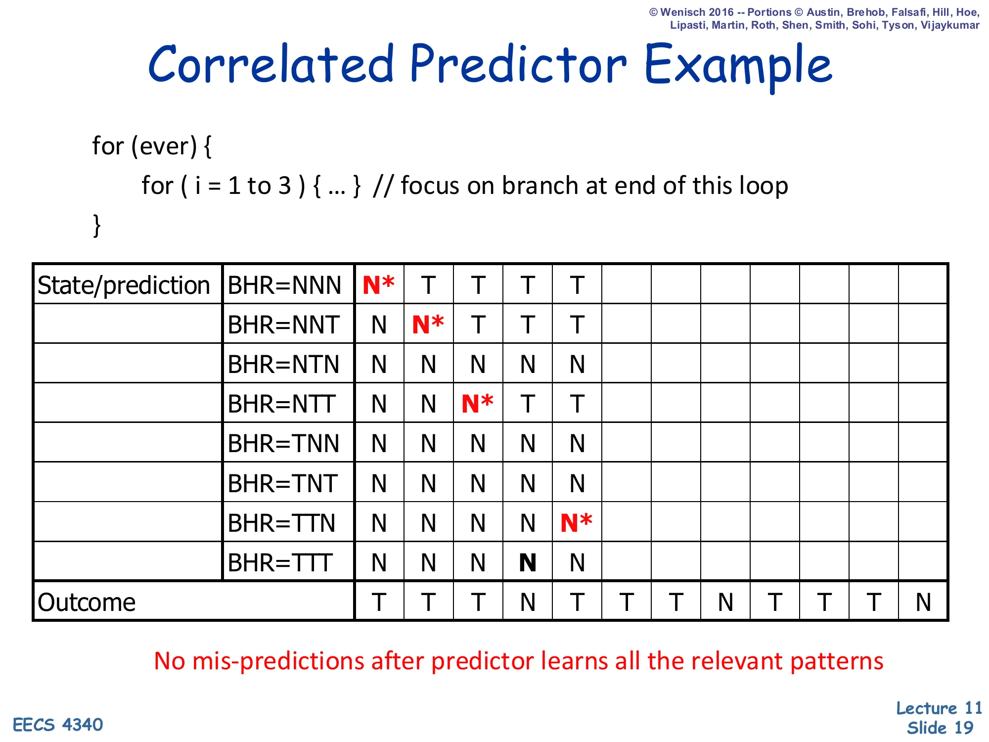
Correlated Predictor Example — Step 5

Slide 19

Show slide text

Correlated Predictor Example

for (ever) {
  for (i = 1 to 3) { ... }   // focus on branch at end of this loop
}

State/prediction
BHR=NNN	N*	T	T	T	T
BHR=NNT	N	N*	T	T	T
BHR=NTN	N	N	N	N	N
BHR=NTT	N	N	N*	T	T
BHR=TNN	N	N	N	N	N
BHR=TNT	N	N	N	N	N
BHR=TTN	N	N	N	N	N*
BHR=TTT	N	N	N	N	N
Outcome	T	T	T	N	T

No mis-predictions after predictor learns all the relevant patterns

Step 5: the BHR has shifted to TTN, so we now consult that row, which still contains N. The actual outcome will be T (we are starting a fresh inner-loop iteration), so this cell will be a misprediction and then flip to T. Each of the eight history rows must be touched at least once before the predictor is fully trained. Because the outcome stream has period 4 (TTTN), only four of the eight rows ever appear in steady state — NNT, NTT, TTT, TTN — so the other four rows will never be looked up after warm-up and their initial-N values do not matter. After a few more iterations the predictor reaches the steady state shown on the next slide where every consulted row holds exactly the right answer.

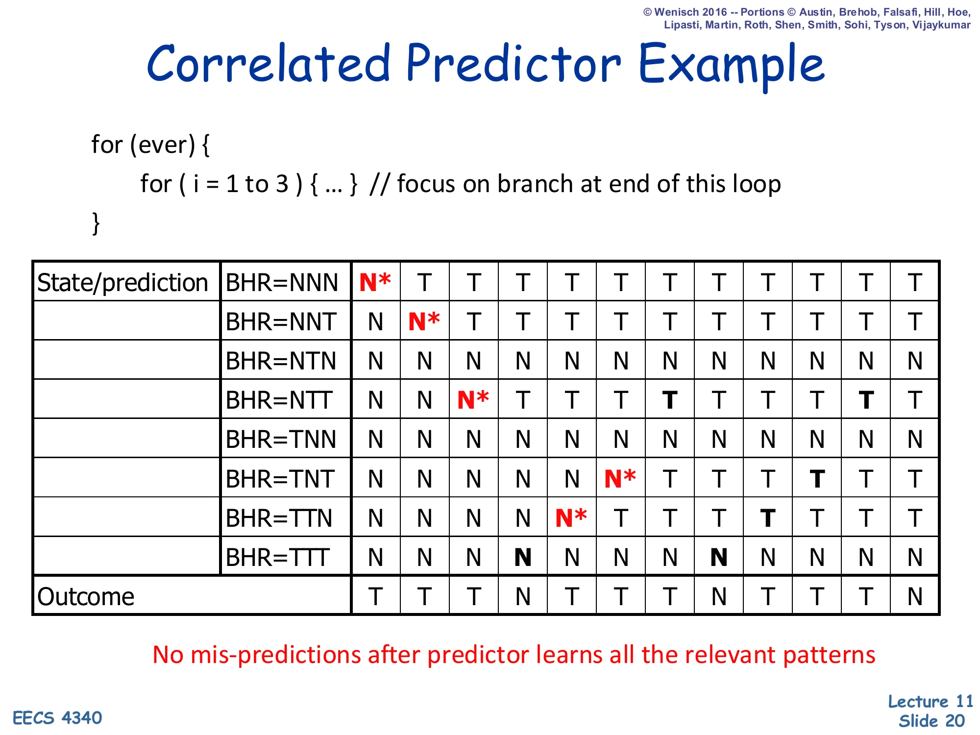
Correlated Predictor Example — Convergence

Slide 20

Show slide text

Correlated Predictor Example

for (ever) {
  for (i = 1 to 3) { ... }   // focus on branch at end of this loop
}

Fully populated table after several iterations (each row records the trajectory of its 1-bit prediction across all 12 cycles of the outcome stream T T T N T T T N T T T N). Active patterns now correctly predict every outcome.

No mis-predictions after predictor learns all the relevant patterns

After enough iterations the four “active” rows have settled at: NNT → T, NTT → T, TTT → N, TTN → T. Each of these rows correctly predicts the single outcome that always follows that history pattern, so the predictor reaches 100% accuracy in steady state. The four “unused” rows (NNN, NTN, TNN, TNT) keep whatever values they last held; they never get consulted because the BHR never reaches those bit-strings under this workload. This is the classic illustration of why a correlated predictor with a 3-bit BHR captures a 4-cycle inner loop perfectly — and conversely why short BHRs are dangerous on inputs whose periodicity exceeds the BHR length: rows from different phases collide and the predictor oscillates instead of converging.

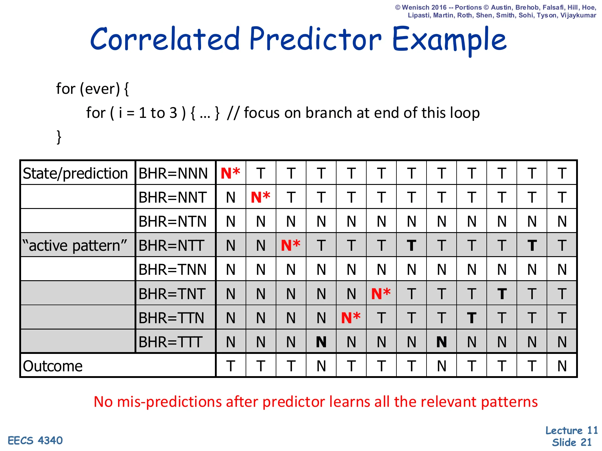
Correlated Predictor Example — Active Patterns

Slide 21

Show slide text

Correlated Predictor Example

Same fully-populated table as the previous slide, with the “active patterns” highlighted: the four rows BHR ∈ {NNT, NTT, TTN, TTT} are shaded because they are the only histories that occur in the steady-state outcome stream TTTN TTTN ....

The other four rows (NNN, NTN, TNN, TNT) are dead rows — they hold whatever value happened to be installed during warm-up but are never consulted again.

No mis-predictions after predictor learns all the relevant patterns

The shaded rows are the predictor’s working set in steady state. Two implications matter for the rest of the lecture: (1) most rows of a per-(PC, history) table are wasted for any given branch — only one history bit-string per branch “phase” is ever live at a time — which motivates the BHT-utilisation argument later for hybrid predictors; and (2) a longer BHR is not always better, because each extra bit doubles the size of the table while only marginally increasing the chance that a still-longer pattern is captured. The active-pattern picture is therefore the right way to think about correlated predictors: the table appears huge on paper, but the dynamic working set is small and concentrated, and the rest of the lecture (gshare, hybrid, TAGE) is largely about picking which table to train and consult on each branch.

Global Branch Prediction

Slide 22

Show slide text

Global Branch Prediction

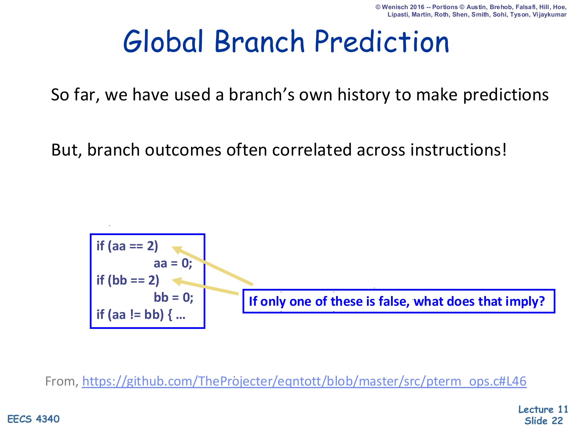
So far, we have used a branch’s own history to make predictions.

But, branch outcomes often correlated across instructions!

if (aa == 2)
  aa = 0;
if (bb == 2)
  bb = 0;
if (aa != bb) { ... }

If only one of these is false, what does that imply?

From https://github.com/TheProjecter/eqntott/blob/master/src/pterm_ops.c#L46

The slide motivates global history with a textbook example from the SPEC eqntott benchmark. The first two ifs zero out aa and bb when they equal 2. So if exactly one of the first two branches is not taken (i.e. one variable equalled 2 and got zeroed while the other did not), then aa != bb is guaranteed to be true: one of them is 0, the other is whatever non-2 value it was, so they differ. The third branch is therefore perfectly determined by the outcomes of the first two branches — but a per-PC predictor for the third branch cannot see that, because each branch only sees its own history. A global branch history register that records the last k outcomes across all dynamic branches — not just this one — exposes the correlation directly, and the same PHT lookup mechanism can use it to capture inter-branch dependencies. This is the conceptual leap that motivates gshare and TAGE.

Global Prediction Implementation

Slide 23

Show slide text

Global Prediction Implementation

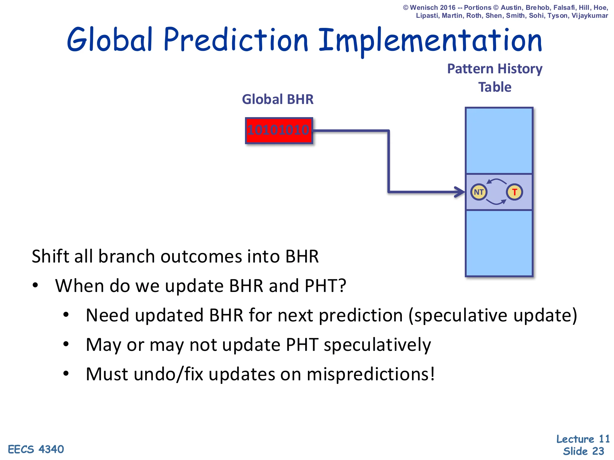
Diagram: a single Global Branch History Register (BHR) holding the bit-string 10101010 indexes into a Pattern History Table whose entry is a 2-state NT ↔ T counter.

Shift all branch outcomes into BHR

• When do we update BHR and PHT?
  • Need updated BHR for next prediction (speculative update)
  • May or may not update PHT speculatively
  • Must undo/fix updates on mispredictions!

Global prediction needs a single shared shift register — the Global BHR — that captures the trajectory of the entire program’s control flow. Every prediction is indexed by this register (often XORed with the PC, as in gshare). The implementation question is when to update the BHR and PHT. The BHR has to be updated speculatively at predict time, because the very next branch in the same fetch group needs its successor’s outcome already shifted in to look up the right PHT row. The PHT can be updated either speculatively (lower latency, but wrong on misprediction) or only at commit (correct, but stale). On a mispredicted branch the BHR has to be rolled back to the value it held before the wrong-path branch — which means the front end has to checkpoint the BHR on every prediction, much like the reorder buffer checkpoints architectural state for precise interrupts.

Correlated Predictor Design Space

Slide 24

Show slide text

Correlated Predictor Design Space

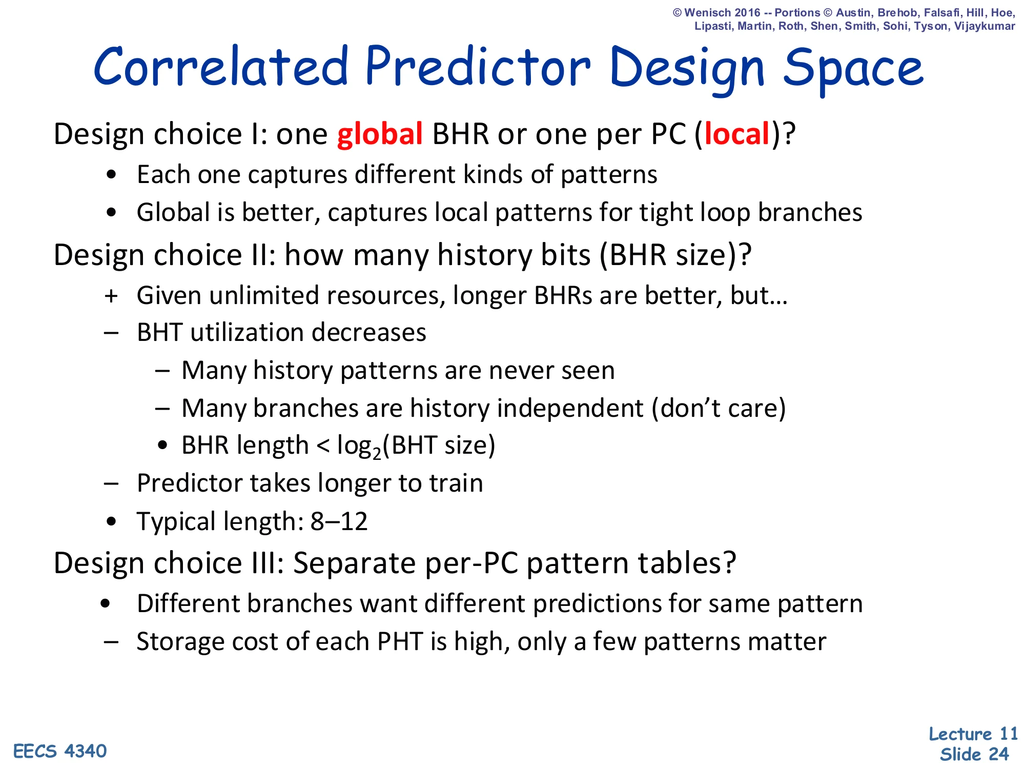
Design choice I: one global BHR or one per PC (local)?

• Each one captures different kinds of patterns
• Global is better, captures local patterns for tight loop branches

Design choice II: how many history bits (BHR size)?

• Given unlimited resources, longer BHRs are better, but…
• BHT utilization decreases
  • Many history patterns are never seen
  • Many branches are history independent (don’t care)
  • BHR length < $\log_2(\text{BHT size})$
• Predictor takes longer to train
• Typical length: 8–12

Design choice III: Separate per-PC pattern tables?

• Different branches want different predictions for same pattern
• Storage cost of each PHT is high, only a few patterns matter

Three orthogonal design choices define every correlated predictor in the literature. (I) Global vs per-PC BHR: a global BHR captures cross-branch correlation (the eqntott example) and also incidentally captures local loop-back patterns, because tight loops dominate the global stream; per-PC BHRs capture only local patterns but are noise-free for the branch in question. (II) BHR length is a sweet-spot problem: too short and patterns alias, too long and the BHT is mostly unused (the active-patterns observation from earlier) and the predictor takes longer to warm up. The constraint BHR length < log₂(BHT size) says that even an unbounded BHR cannot help once it exceeds the table’s index width. (III) Whether to split the PHT per-PC: separate tables let two branches with different biases consult their own counters, but at high storage cost. These three knobs span the design space {G,P}A{g,p,s} formalised on slide 25.

Taxonomy & Nomenclature [Patt]

Slide 25

Show slide text

Taxonomy & Nomenclature [Patt]

Diagram: branchPC indexes a per-PC Branch History Register table; the selected row holds the bit-string 10101010, which then indexes a per-PC Pattern History Table whose entry is the 2-state NT ↔ T counter.

$\{G,P\} A \{g,p,s\}$

• $G$ / $P$: Global or Per-PC BHR
• $g$ / $p$ / $s$: global, per-PC, or set PHT

Yeh and Patt’s taxonomy uses a four-letter code XAY where the first letter is uppercase G or P (Global or Per-PC BHR), A stands for “Adaptive,” and the third letter is lowercase g, p, or s (global, per-PC, or per-set PHT). So GAg means one global BHR and one global PHT — the design later realised cheaply by gshare. PAp means each branch gets its own BHR and its own PHT — strictly more powerful but storage-prohibitive. GAs and PAs use one PHT per set of branches (typically a hash of the PC), trading per-PC isolation for table size. The next two slides expand the per-PC and global rows of the taxonomy with the original Yeh & Patt diagrams. The taxonomy matters because it gives a vocabulary for talking about real predictors: the Pentium MMX used a per-PC BHR with a global PHT (PAg-like); the Alpha 21264 used a tournament of GAg and a per-PC bimodal — and so on.

Per-PC History (PAg, PAs, PAp)

Slide 26

Show slide text

Per-PC History

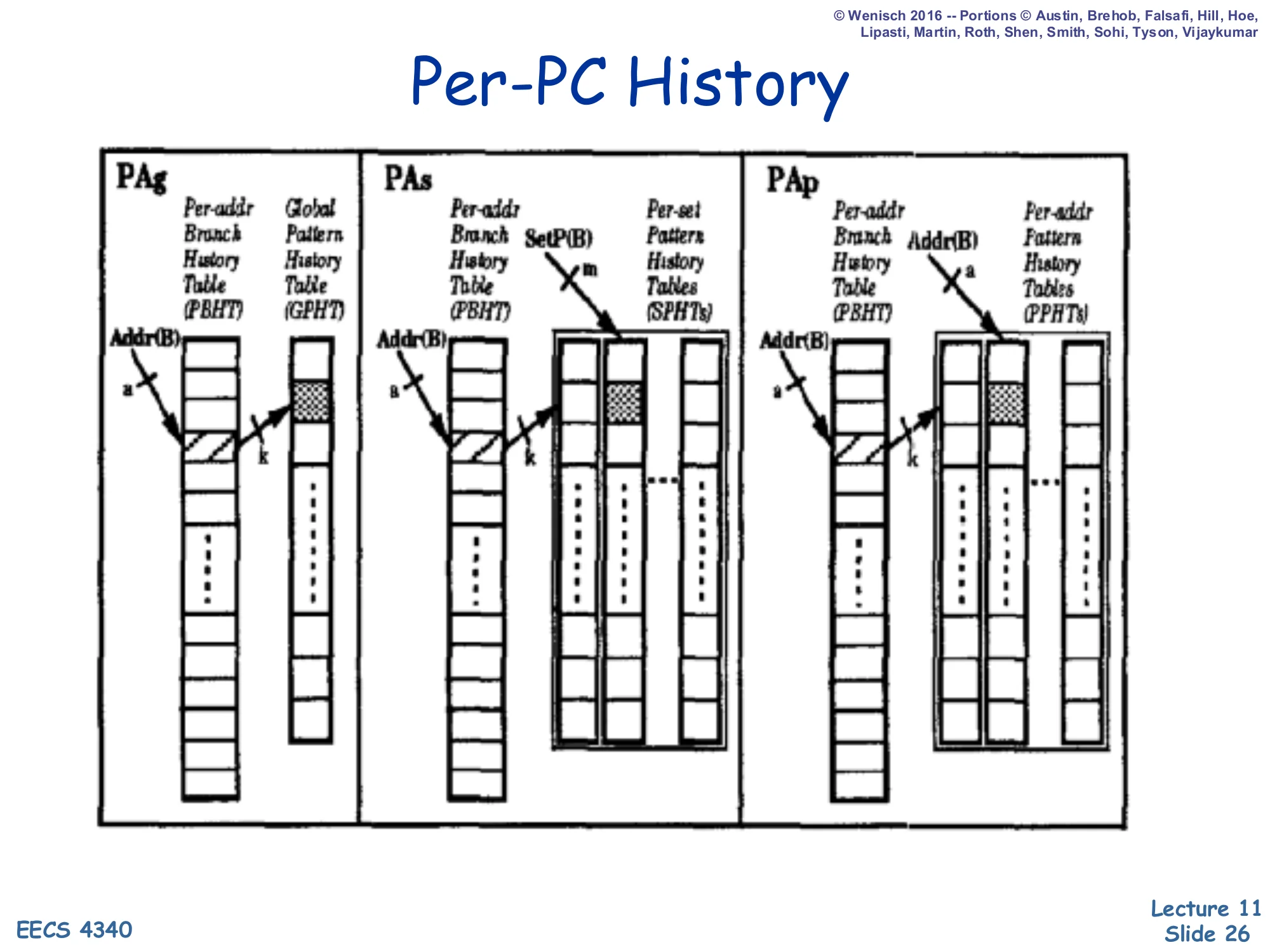
Three side-by-side diagrams from Yeh & Patt:

• PAg: Per-Address Branch History Table (PBHT) → Global Pattern History Table (GPHT). Branch address Addr(B) selects a BHR row of length a; that BHR indexes a single global PHT.
• PAs: PBHT → Per-Set Pattern History Tables (SPHTs). The BHR row plus a function SetP(B) of the branch (m bits) chooses one of several set-shared PHTs.
• PAp: PBHT → Per-Address Pattern History Tables (PPHTs). Each branch gets its own BHR and its own PHT, indexed by Addr(B).

These are the three flavours of Per-PC (P) BHR predictors. PAg keeps a separate history register per branch but pools the prediction counters in a single global PHT; this works well when many branches happen to follow the same pattern shape (e.g. all the loop-exit branches in a hot loop nest). PAs sits in the middle: the PHT is replicated per set of branches, so groups of related branches share counters but unrelated branches get isolation. PAp gives every branch its own BHR and its own PHT — maximum isolation, maximum storage. As an order-of-magnitude rule, PAp’s storage scales with (# branches) × 2^(BHR length), which becomes infeasible for BHR lengths beyond about 6–8 even on small benchmarks. Real hardware therefore almost never implements PAp; it implements PAg or PAs, and uses associativity or hashing tricks to approximate the per-PC isolation that PAp would have given.

Global History (GAg, GAs, GAp)

Slide 27

Show slide text

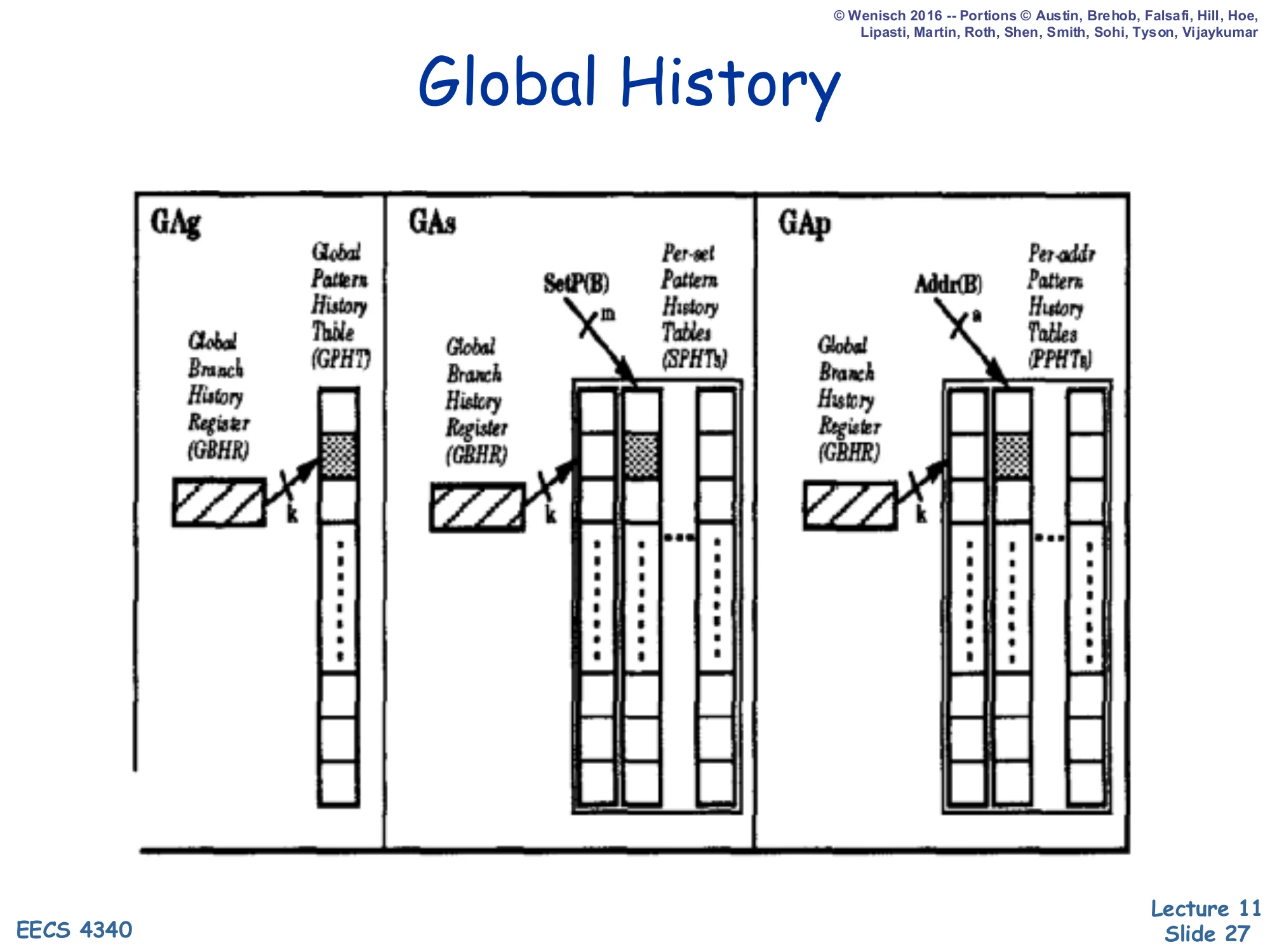
Global History

Three side-by-side diagrams:

• GAg: a single Global Branch History Register (GBHR) of width k directly indexes one Global Pattern History Table (GPHT).
• GAs: GBHR → Per-Set Pattern History Tables (SPHTs), one PHT per set selected by SetP(B) (m bits).
• GAp: GBHR → Per-Address Pattern History Tables (PPHTs), one PHT per branch selected by Addr(B) (a bits).

These are the three flavours of Global (G) BHR predictors. GAg is the simplest design that captures inter-branch correlation: a single global history register and a single PHT shared by every branch. Its weakness is destructive aliasing — two unrelated branches that happen to see the same recent global history will share a counter and may train it in opposite directions. GAs mitigates that by hashing the branch into one of several PHTs (per-set). GAp goes further and gives every branch its own PHT, costing as much storage as PAp. The lecture immediately follows this slide with gshare, which is a remarkably cheap way to approximate GAs/GAp by simply XORing the PC into the global history before indexing — getting the per-branch isolation benefit of GAp at the storage cost of GAg.

Gshare [McFarling]

Slide 28

Show slide text

Gshare [McFarling]

Diagram: branchPC and a Global BHR holding 10101010 are XORed together; the XOR result indexes a single Pattern History Table whose entry is the 2-state NT ↔ T counter.

Cheap way to implement GAs

• Global branch history
• Per-address patterns (sort of)
• Try to make the PHT big enough to avoid collisions

gshare is the predictor that made global-history schemes practical. It indexes a single PHT with branchPC XOR globalBHR, mixing per-branch identity into the global-history index for free. Two branches with the same global history but different PCs land on different PHT rows, giving the per-PC isolation of GAp; two branches with the same PC but different histories also land on different rows, giving the history sensitivity of GAg. The catch is that XOR is not a perfect hash: two distinct (PC, BHR) pairs can collide if their bit-patterns XOR to the same value, so the slide stresses “try to make the PHT big enough to avoid collisions.” Empirically, gshare with a 64 K-entry PHT and a 14-bit BHR hits ~94% accuracy on SPECint, which is the bar that every subsequent design (bi-mode, agree, YAGS, TAGE) had to clear. McFarling’s paper also introduced the combining (hybrid) predictor on the next slide.

Hybrid Predictor

Slide 29

Show slide text

Hybrid Predictor

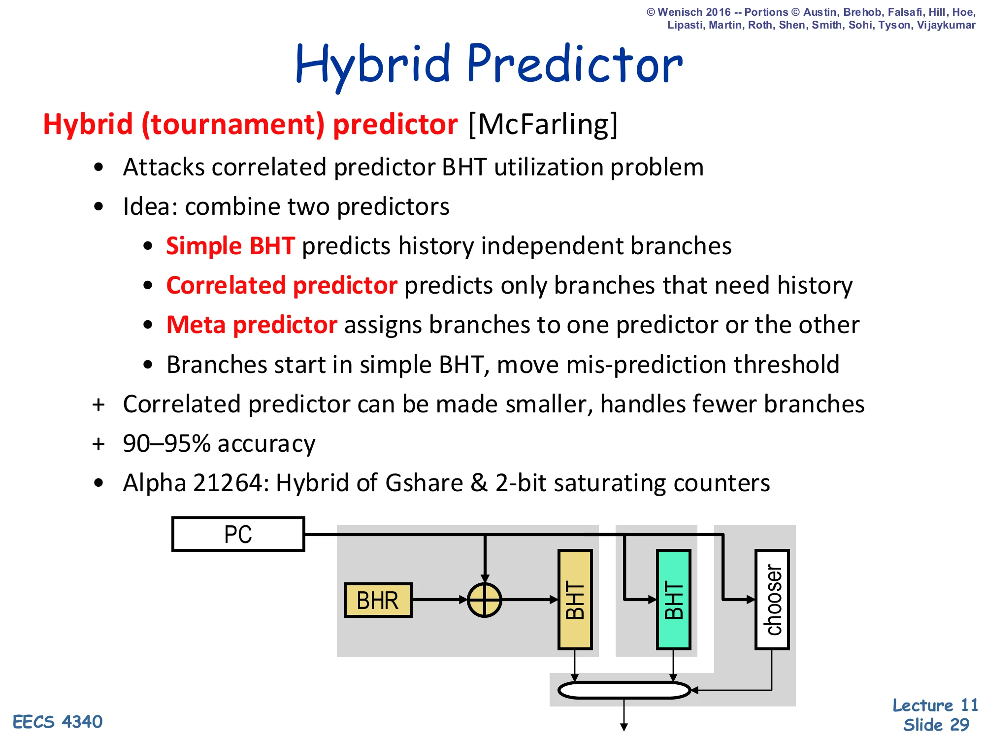
Hybrid (tournament) predictor [McFarling]

• Attacks correlated predictor BHT utilization problem
• Idea: combine two predictors
  • Simple BHT predicts history independent branches
  • Correlated predictor predicts only branches that need history
  • Meta predictor assigns branches to one predictor or the other
  • Branches start in simple BHT, move mis-prediction threshold

• Correlated predictor can be made smaller, handles fewer branches
• 90–95% accuracy

• Alpha 21264: Hybrid of Gshare & 2-bit saturating counters

Diagram: PC fans into a BHT (XORed with BHR before lookup), a second BHT, and a chooser; the two BHT outputs and the chooser pick the final prediction.

A tournament predictor exploits the active-patterns observation: most branches are easy (per-PC bimodal handles them), and only a minority of branches need history. Two predictors run in parallel — one cheap bimodal and one expensive correlated/gshare — and a meta-predictor (itself a table of 2-bit counters indexed by PC) tracks which one has been right more recently for each branch and selects between them. Branches start out being routed to the cheap predictor and only migrate to the correlated one once their misprediction count crosses a threshold. The result is that the correlated PHT can be smaller (because it only has to store entries for hard branches) and accuracy reaches 90–95%. The Alpha 21264, which the slide cites, used a hybrid of gshare and per-PC 2-bit counters — and was a benchmark setter for late-1990s commercial branch prediction.

Towards the State of the Art: TAGE [Seznec]

Slide 30

Show slide text

Towards the state of the art: TAGE [Seznec]

Around 2003:

• 2bcgskew (variant of gshare) was state-of-the-art
  • But, lagging behind neural-inspired predictors for some workloads
• Seznec sought to get the best of both
  • Reasonable implementation cost:
    • Use only global history
    • Medium number of tables
  • In-time response

Around 2003 the strongest published predictor was 2bcgskew, a gshare variant that fed two PHTs whose indexing functions were mutually skewed to break aliasing. Neural-inspired predictors (Jiménez & Lin’s perceptron predictor, 2001) were even more accurate on some workloads, but their dot-product computation was too slow to deliver a prediction in a single fetch cycle. Seznec’s TAGE — TAgged GEometric history-length — set out to recover neural-class accuracy with a more pipelineable design: only global history (no per-PC BHRs), a medium number of tagged tables (4–12 in practice), and crucially an “in-time” response: each table can be looked up in parallel and the highest-priority hit is selected combinatorially. TAGE remains the basis of every modern champion in the Championship Branch Prediction (CBP) benchmark and is the front-end predictor in many recent commercial cores.

The Basis: A Multiple-Length Global History Predictor

Slide 31

Show slide text

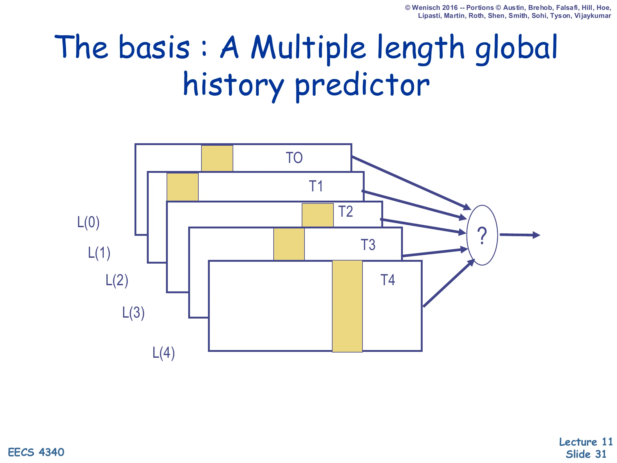
The basis: A Multiple-length global history predictor

Diagram: five tables T0, T1, T2, T3, T4 stacked back-to-front, each consulted with a different global-history length L(0) < L(1) < L(2) < L(3) < L(4). All five outputs feed a ? selector that produces the final prediction.

The history lengths grow geometrically (typically $L(i) = L(0) \cdot \alpha^i$ with $\alpha \approx 2$).

TAGE’s central insight is that different branches need different history lengths. Some branches correlate with the immediately preceding branch (history length 1–4); others depend on a control-flow event from dozens of branches earlier (history length 100+). A single fixed-length BHR has to compromise. TAGE instead keeps a bank of tables T0…Tn, where each Ti is indexed using a different history length L(i). The lengths grow geometrically (the “GE” in TAGE) — typically L(i) = L(0)·α^i with α≈2 — so a small number of tables covers a wide range, e.g. 4, 8, 16, 32, 64, 128 history bits. T0 is the base predictor (a plain bimodal — no history). For any given branch the predictor picks the table with the longest matching history. The next slide shows the tagged matching mechanism that makes this possible.

TAGE — Tagged Geometric History Length

Slide 32

Show slide text

TAGE [Seznec]

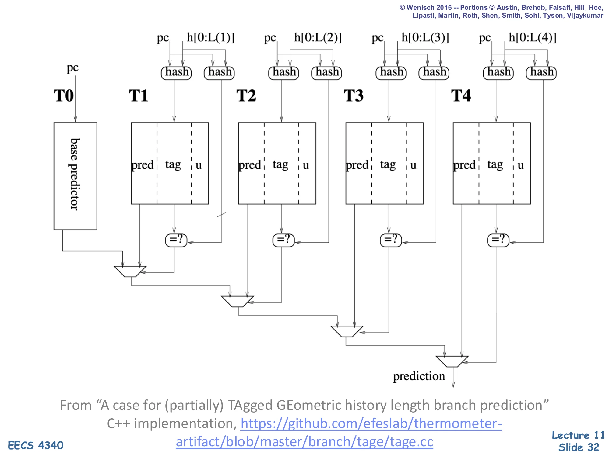
Full TAGE diagram: a base predictor T0 (indexed by PC alone) plus four tagged tables T1, T2, T3, T4. Each Ti is indexed by a hash of the PC and the global history h[0:L(i)] where the lengths $L(1) < L(2) < L(3) < L(4)$ grow geometrically. Each tagged entry stores three fields:

• pred — the prediction (saturating counter)
• tag — a hash of (PC, history) used to detect aliasing
• u — a useful bit

A bank of =? comparators per table checks whether the stored tag matches; the rightmost (longest-history) table whose tag matches wins the priority mux at the bottom and supplies the final prediction. If no tagged table matches, T0’s base prediction is used.

From “A case for (partially) TAgged GEometric history length branch prediction” — C++ implementation: https://github.com/efeslab/thermometer-artifact/blob/master/branch/tage/tage.cc

TAGE’s defining feature is that every entry in T1…Tn carries a tag — a hash of the (PC, history) used to look it up — and a comparator decides whether the entry actually matches. So each table answers two questions at once: does my row match this (PC, history)? and if so, what’s the prediction? On a branch lookup all tables fire in parallel; the priority mux at the bottom picks the table with the longest matching history, falling back to T0 if no tagged table matches. This is the “partially tagged” idea: T0 is untagged (so it always answers), but every higher table is tagged so that it can refuse to predict when it has not seen this exact (PC, history) before. The u bit is a usefulness counter that controls allocation on misprediction: a longer-history entry only displaces a shorter one if it has been useful, so frequently-correct short-history entries are not constantly evicted by experimental long-history allocations. This combination — geometric lengths, partial tagging, useful-bit allocation — is what gives TAGE its ~96–98% accuracy on SPEC.

BP Implementation Challenges

Slide 33

Show slide text

BP Implementation Challenges

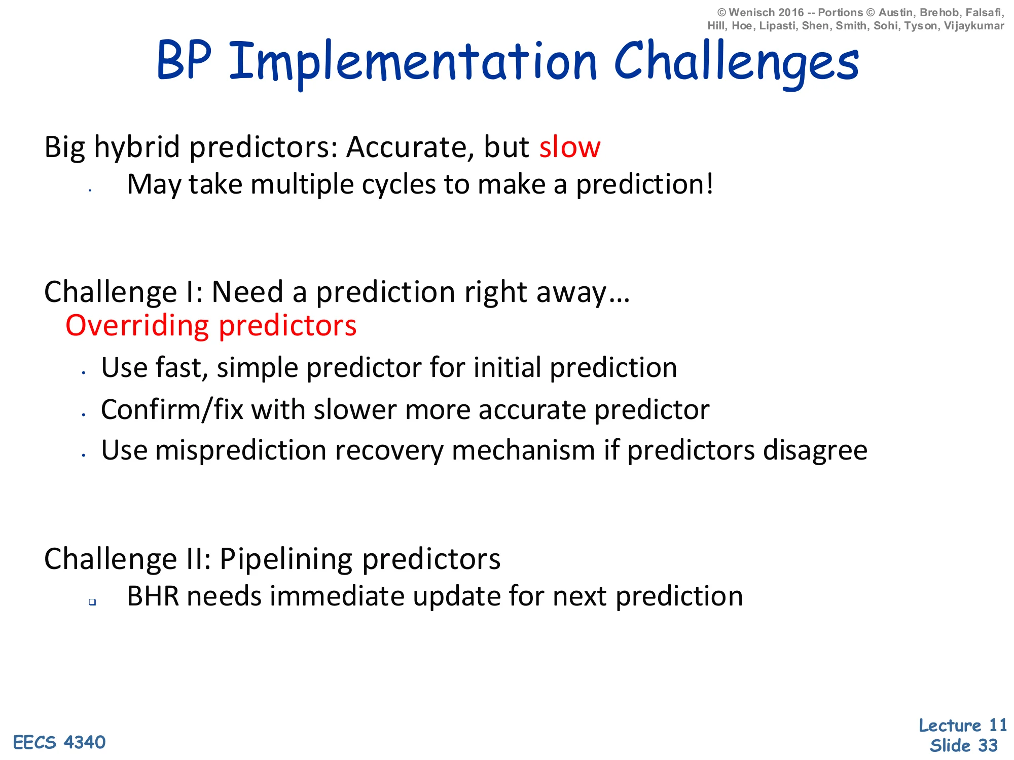
Big hybrid predictors: Accurate, but slow

• May take multiple cycles to make a prediction!

Challenge I: Need a prediction right away…

• Overriding predictors
  • Use fast, simple predictor for initial prediction
  • Confirm/fix with slower more accurate predictor
  • Use misprediction recovery mechanism if predictors disagree

Challenge II: Pipelining predictors

• BHR needs immediate update for next prediction

Accuracy is not free: a TAGE-class predictor can take 2–3 cycles to deliver a prediction, but the front end has to fetch a new instruction every cycle. The classic solution is an overriding predictor: a tiny, fast predictor (a single-cycle bimodal or BTB) supplies an initial prediction every cycle, while the big predictor runs in the background. When the big predictor finishes 2–3 cycles later, its answer is compared to the fast one; if they disagree the in-flight instructions on the wrong path are squashed using the same recovery machinery used for branch mispredictions. The second challenge — pipelining the predictor — is even subtler. The BHR must be updated speculatively the cycle a branch is predicted, because the next branch needs the updated history. So on every prediction the predictor checkpoints the BHR, and on every misprediction it rolls back to the snapshot of the correct branch — analogous to what the reorder buffer does for architectural state.

Mis-speculation Recovery

Slide 34

Show slide text

Mis-speculation Recovery

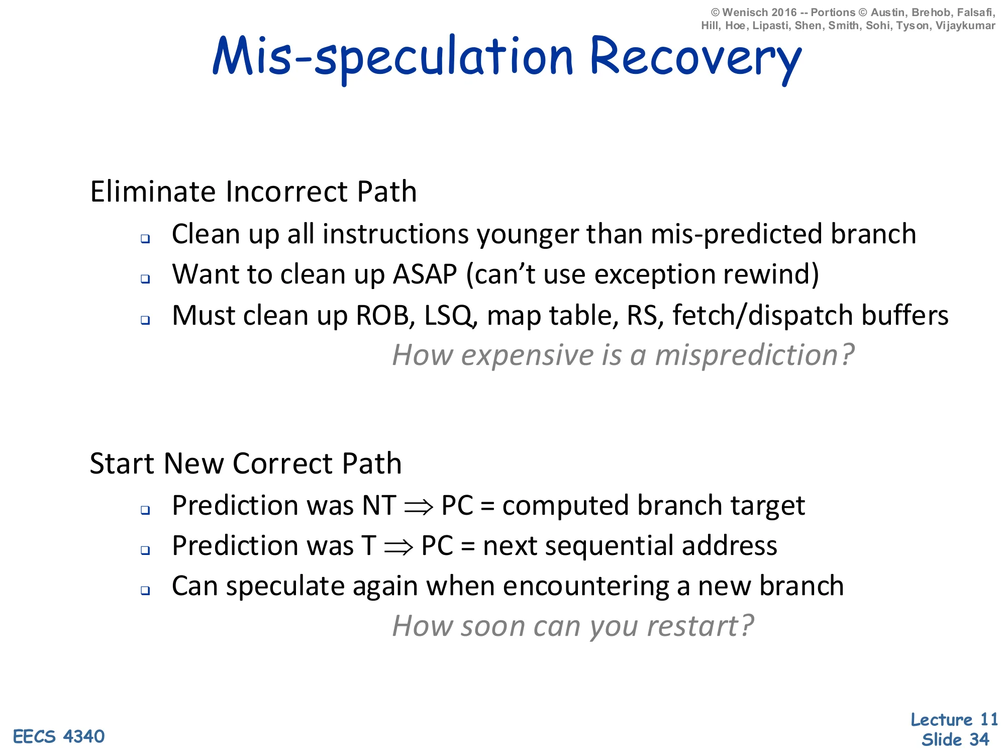
Eliminate Incorrect Path

• Clean up all instructions younger than mis-predicted branch
• Want to clean up ASAP (can’t use exception rewind)
• Must clean up ROB, LSQ, map table, RS, fetch/dispatch buffers
  • How expensive is a misprediction?

Start New Correct Path

• Prediction was NT ⇒ PC = computed branch target
• Prediction was T ⇒ PC = next sequential address
• Can speculate again when encountering a new branch
  • How soon can you restart?

Once a branch resolves and turns out to have been mispredicted, the core has to undo every effect of the wrong-path instructions and restart fetch on the correct path. “Cannot use exception rewind” means we cannot afford to wait until the branch retires from the reorder buffer (the way an interrupt-induced flush works) — that would take dozens of cycles. Instead, recovery has to be triggered the moment branch resolution discovers the misprediction, ASAP. The cleanup list is comprehensive: ROB entries for younger instructions, load-store queue entries, the rename map table (so freed physical registers are reclaimed), reservation stations, the fetch and dispatch buffers in the front end. Once everything is squashed the new fetch PC is set to the other path: if the prediction was “not taken” the correct path is the computed target; if it was “taken” the correct path is the fall-through. The next two slides describe the branch-stack mechanism that makes this single-cycle recovery possible.

Fast Branch Recovery

Slide 35

Show slide text

Fast Branch Recovery

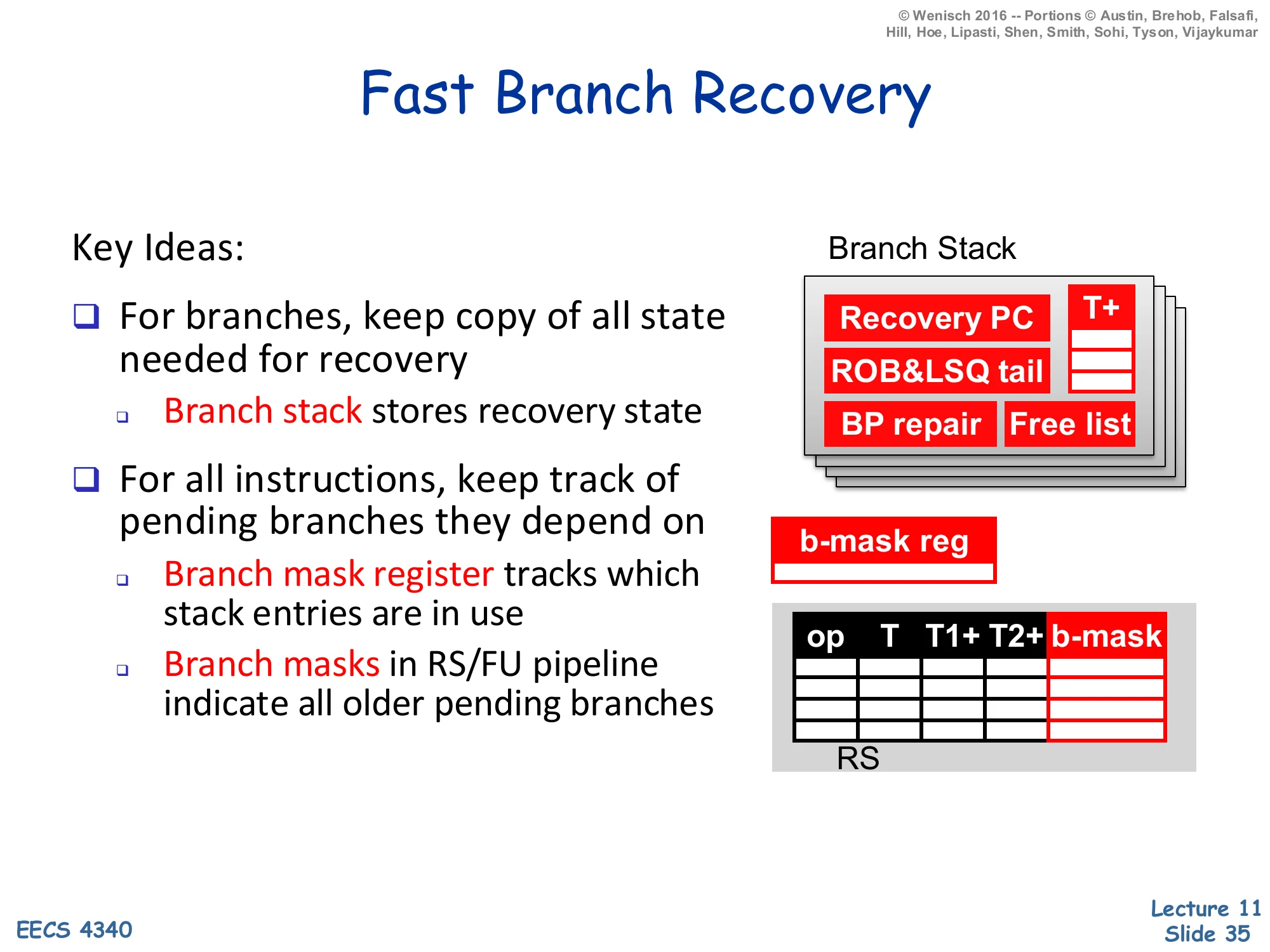
Key Ideas:

• For branches, keep copy of all state needed for recovery
  • Branch stack stores recovery state
• For all instructions, keep track of pending branches they depend on
  • Branch mask register tracks which stack entries are in use
  • Branch masks in RS/FU pipeline indicate all older pending branches

Diagram: a Branch Stack of entries each holding Recovery PC, ROB&LSQ tail, BP repair, Free list, with a T+ pointer indicating the most recent allocation. A b-mask reg is a bit-vector with one bit per active stack entry. The reservation station has columns op | T | T1+ | T2+ | b-mask so each in-flight instruction carries a copy of the b-mask snapshot at its dispatch.

Fast recovery works because the core treats every speculative branch as a checkpoint. The branch stack is a small SRAM with one entry per outstanding branch; each entry stores everything needed to roll back to the predicted-correct state at that branch — the recovery PC, the ROB and LSQ tail pointers, the predictor repair info (BHR/PHT snapshots), and the rename free list. Concurrently, a branch mask register is a bit vector with one bit per branch-stack entry (so 4 bits if the stack is 4-deep). When a branch is dispatched, a fresh stack slot is allocated and the corresponding mask bit is set; every younger instruction copies that mask into its RS entry. On a misprediction, the core looks up the offending branch’s stack entry, restores everything from it, and squashes every RS/FU entry whose b-mask bit for that branch is set. The whole recovery happens in essentially one cycle, because no traversal of the reorder buffer is required — the b-mask flags identify all dependent instructions in parallel.

Fast Branch Recovery — Dispatch Stage

Slide 36

Show slide text

Fast Branch Recovery — Dispatch Stage

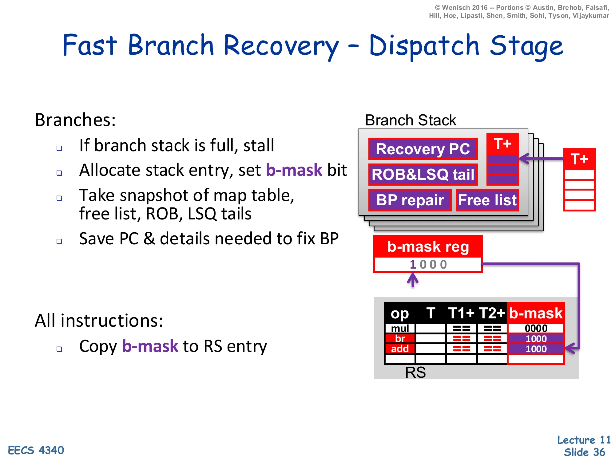
Branches:

• If branch stack is full, stall
• Allocate stack entry, set b-mask bit
• Take snapshot of map table, free list, ROB, LSQ tails
• Save PC & details needed to fix BP

All instructions:

• Copy b-mask to RS entry

Diagram: dispatching a branch allocates the next free branch-stack entry (showing Recovery PC, ROB&LSQ tail, BP repair, Free list), sets the leading 1 in the b-mask reg (= 1000), and the value 1000 is then propagated to the b-mask columns of two younger RS entries (br and add in the table).

At dispatch time, every instruction carries a snapshot of the current branch mask register, which encodes “which speculative branches am I younger than?” For non-branch instructions, the mask is just copied verbatim into the reservation-station entry’s b-mask field. For branches, three additional things happen: (1) a free entry on the branch stack is allocated (or the pipeline stalls if the stack is full — the worked example uses a 4-deep stack), (2) the branch’s mask bit is set in the live b-mask register so all subsequent instructions inherit it, and (3) a snapshot of the current rename map, free list, ROB tail, and LSQ tail is captured into the new stack entry along with the recovery PC and the predictor-repair info. The slide’s example shows two younger instructions (br and add) inheriting 1000 because they are younger than the branch that allocated bit-0 of the mask. On misprediction the recovery hardware will flash-clear every RS entry whose copy of the bit is set.

Fast Branch Recovery — Branch Resolution: Mispredict

Slide 37

Show slide text

Fast Branch Recovery — Branch Resolution — Mispredict

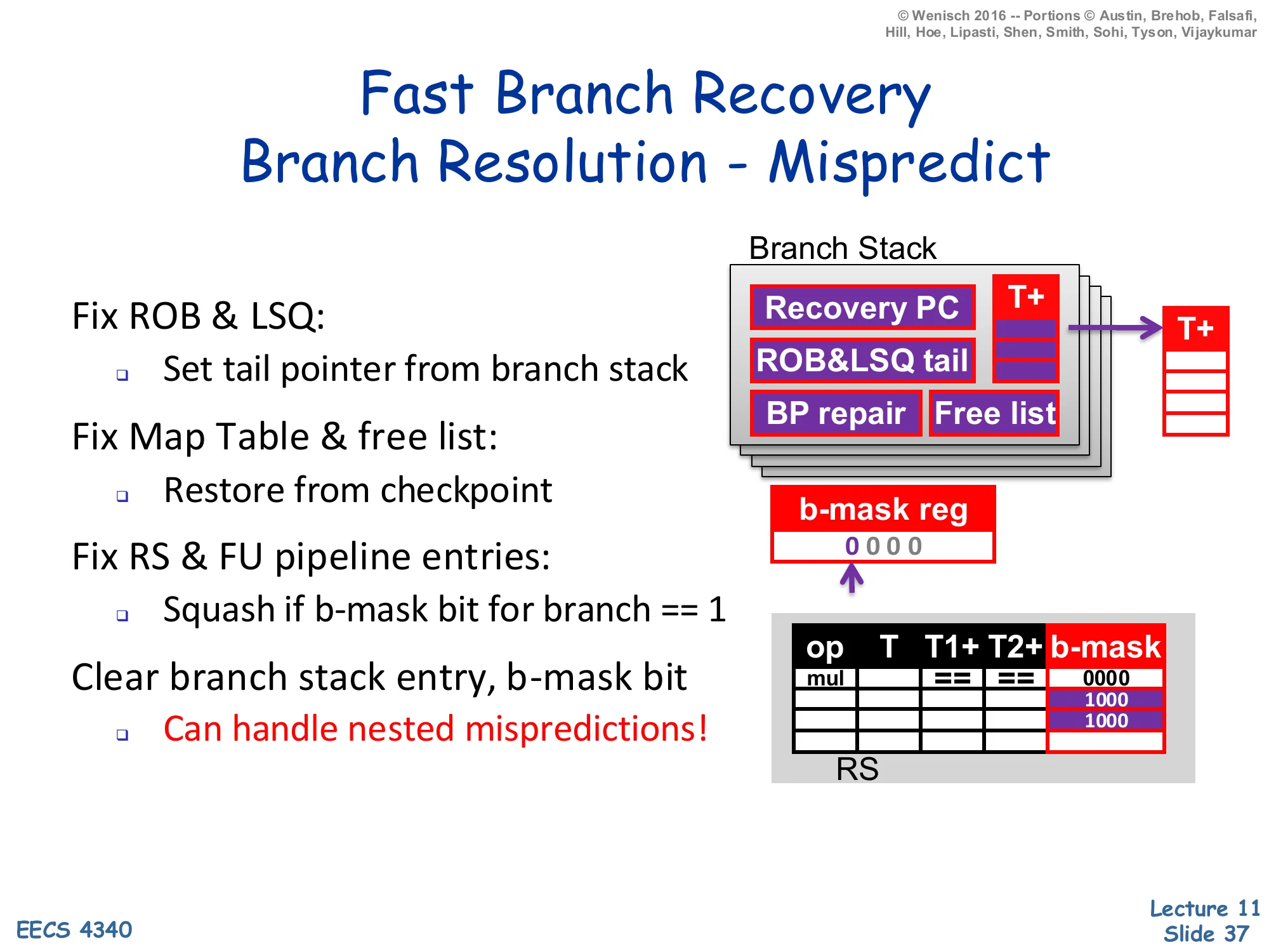
Fix ROB & LSQ: Set tail pointer from branch stack

Fix Map Table & free list: Restore from checkpoint

Fix RS & FU pipeline entries: Squash if b-mask bit for branch == 1

Clear branch stack entry, b-mask bit

• Can handle nested mispredictions!

Diagram: after resolution the b-mask register is reset to 0000, the branch stack entry is freed, and any RS entries whose stored b-mask had the offending bit set are squashed (shown as cleared rows).

On misprediction, the offending branch’s stack entry is read out and used to restore four pieces of state in parallel: ROB and LSQ tails are rewound to the snapshot, the rename map and free list are restored from their checkpoint (so all wrong-path physical-register allocations are reclaimed), the predictor’s BHR/PHT updates are repaired, and the front end starts fetching from the recovery PC. Concurrently every reservation station and FU pipeline entry whose b-mask bit for this branch is 1 is flash-squashed — a single AND with the resolved-branch’s mask bit identifies every in-flight wrong-path instruction without any traversal. The mask bit is then cleared globally and the stack slot is freed for re-use. The crucial “can handle nested mispredictions” claim follows because each branch has its own independent mask bit: if branch A is younger than branch B and both are wrong, recovering from A first squashes only A-and-younger instructions, leaving B and B’s older but A-younger context intact for B’s subsequent recovery.

Fast Branch Recovery — Branch Resolution: Correct Prediction

Slide 38

Show slide text

Fast Branch Recovery — Branch Resolution — Correct Prediction

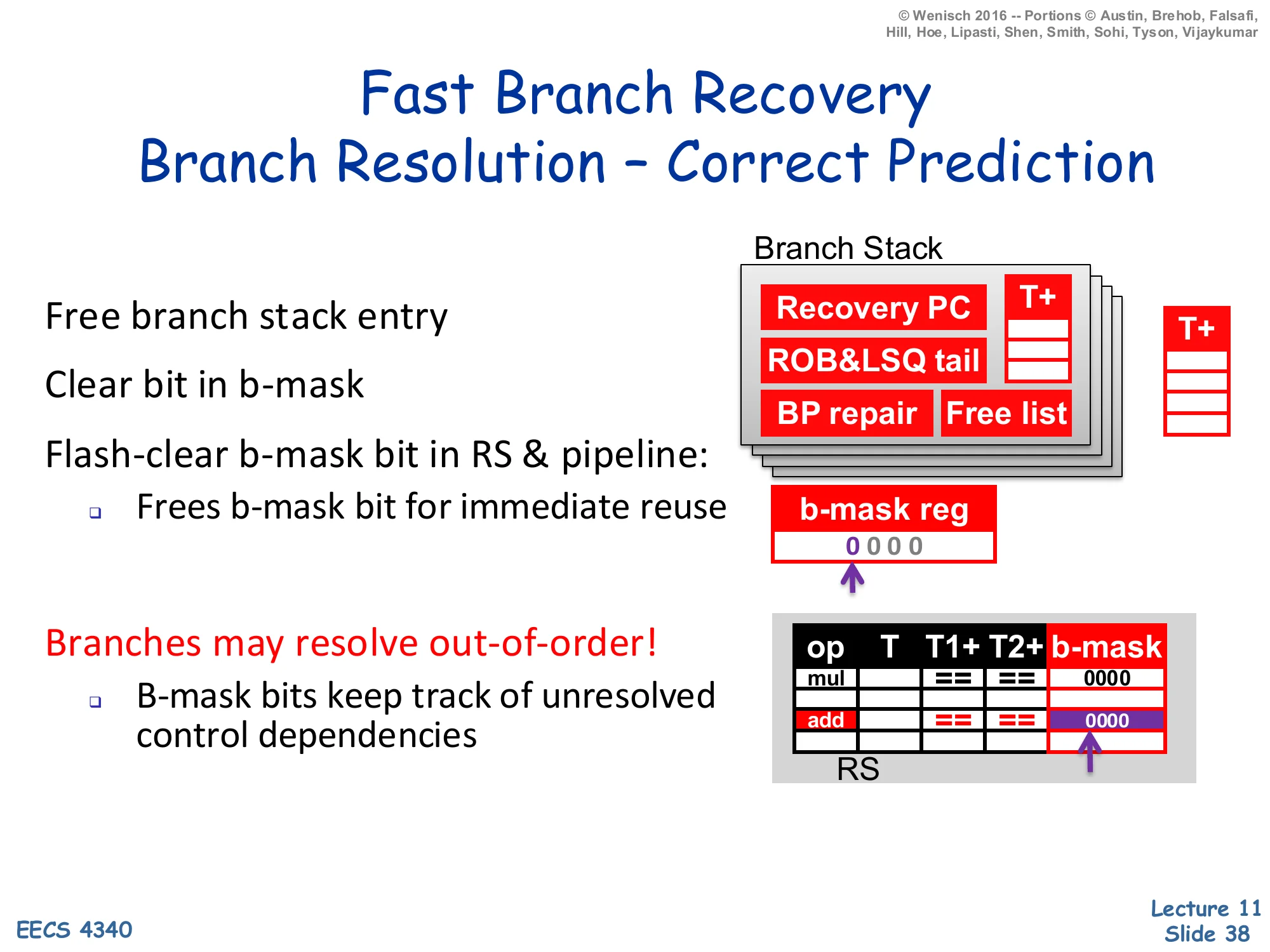
Free branch stack entry

Clear bit in b-mask

Flash-clear b-mask bit in RS & pipeline:

• Frees b-mask bit for immediate reuse

Branches may resolve out-of-order!

• B-mask bits keep track of unresolved control dependencies

Diagram: same branch-stack and RS layout as previous slides, but on a correct resolution every RS entry’s b-mask column has its corresponding bit cleared (0000).

On a correctly-predicted branch, recovery is unnecessary, but the bookkeeping still needs to happen: the stack slot is freed, the live b-mask register clears that branch’s bit, and every RS and FU pipeline entry that had set that bit gets it flash-cleared in parallel. “Flash-clear” here is just ANDing the b-mask column with the inverse of the resolved branch’s bit, which is a single broadcast wire — it does not require any per-entry sequencing. Importantly, branches resolve out-of-order in a real OoO core: branch B can resolve before branch A even though A was dispatched first, because A might be waiting on a long-latency dependence. The b-mask is exactly the right encoding for this: each instruction’s mask records which outstanding branches it depends on, regardless of program order, so out-of-order resolution just clears bits asynchronously without disturbing instructions that depend on still-unresolved older branches.

Wide Instruction Fetch Issues

Slide 39

Show slide text

Wide Instruction Fetch Issues

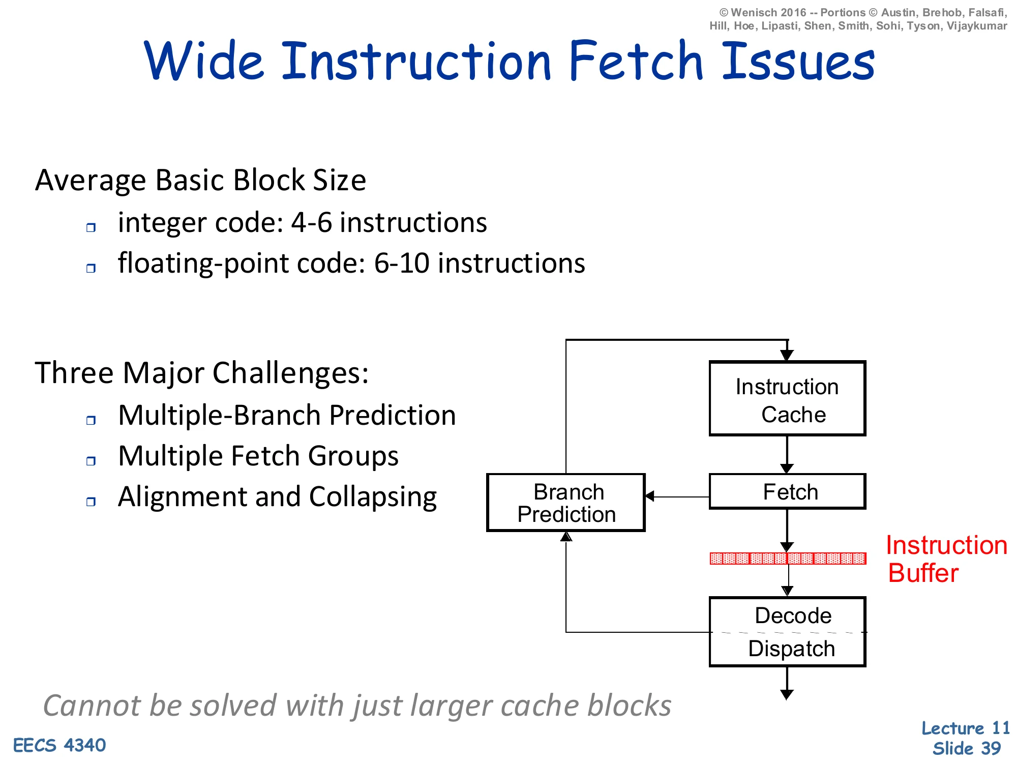
Average Basic Block Size

• integer code: 4–6 instructions
• floating-point code: 6–10 instructions

Three Major Challenges:

• Multiple-Branch Prediction
• Multiple Fetch Groups
• Alignment and Collapsing

Diagram: a front end loop showing Instruction Cache → Fetch → Instruction Buffer → Decode/Dispatch, with a Branch Prediction unit feeding back into Fetch.

Cannot be solved with just larger cache blocks

Wide superscalar processors want to fetch 4, 8, or even 16 instructions per cycle. But basic blocks are short — typically 4–6 instructions for integer code and 6–10 for FP — so a fetch group of 8 instructions usually contains at least one branch. The slide identifies three challenges that simply enlarging the cache block does not solve. (1) Multiple-branch prediction: more than one taken branch may sit inside a single fetch window, and predicting them sequentially serialises the front end. (2) Multiple fetch groups: the predicted-taken branch’s target lives in a different cache line, so we need to access two (or three) lines this cycle. (3) Alignment and collapsing: the useful instructions may not start at a cache-line boundary and may be scattered across multiple lines, so a crossbar is needed to compact them into a contiguous fetch buffer. The next slides walk through each challenge and the trace cache solution that addresses all three at once.

Wide Fetch — Sequential Instructions

Slide 40

Show slide text

Wide Fetch — Sequential Instructions

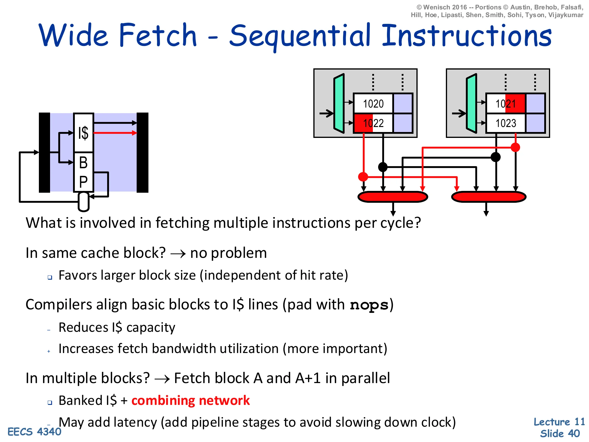
Left: a small front-end pipeline icon showing I$ + BP feeding the fetch stage.

Right: two sets of two-line cache blocks. In the first set the cache lines hold instructions starting at addresses 1020 and 1022 — the desired four sequential instructions span two lines, but they sit at the boundary so a simple combining network can stitch them together. In the second set the desired window starts at 1021 and 1023 and the desired bytes are scattered, illustrating misaligned fetch.

What is involved in fetching multiple instructions per cycle?

In same cache block? → no problem

• Favors larger block size (independent of hit rate)

Compilers align basic blocks to I$ lines (pad with nops)

• Reduces I$ capacity

• Increases fetch bandwidth utilization (more important)

In multiple blocks? → Fetch block A and A+1 in parallel

• Banked I$ + combining network
• May add latency (add pipeline stages to avoid slowing down clock)

If the desired N instructions all live in the same I-cache block, fetching them in one cycle is trivial — read out the block and select the right N words. So larger blocks help wide fetch directly, independent of their hit-rate effect. Compilers can further help by aligning basic blocks to cache-line boundaries with NOP padding; this wastes I-cache capacity (the NOPs are instructions that get fetched and decoded for nothing) but raises fetch-bandwidth utilisation, which the slide notes is the more important effect on wide cores. When the window straddles two blocks the I-cache is banked so block A and block A+1 can be read in parallel from independent SRAM arrays, and a combining network (a multiplexer crossbar) selects the right bytes from each. The trade-off is latency: the combining stage adds wires and muxes, which may force an extra pipeline stage to keep the clock period short. None of this helps with non-sequential fetches caused by taken branches — that is the topic of the next slide.

Wide Fetch — Non-sequential

Slide 41

Show slide text

Wide Fetch — Non-sequential

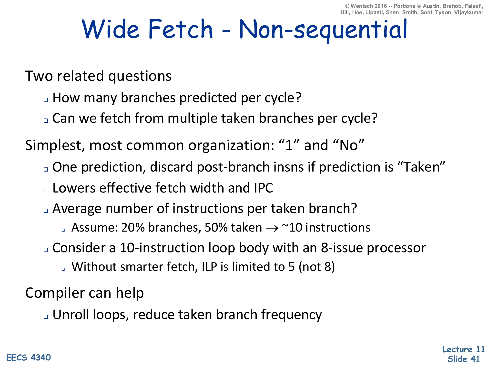
Two related questions:

• How many branches predicted per cycle?
• Can we fetch from multiple taken branches per cycle?

Simplest, most common organization: “1” and “No”

• One prediction, discard post-branch insns if prediction is “Taken”
• Lowers effective fetch width and IPC
• Average number of instructions per taken branch?
  • Assume: 20% branches, 50% taken → ~10 instructions
• Consider a 10-instruction loop body with an 8-issue processor
  • Without smarter fetch, ILP is limited to 5 (not 8)

Compiler can help

• Unroll loops, reduce taken branch frequency

Most commercial cores predict one branch per cycle and discard everything in the fetch group past a predicted-taken branch. The arithmetic on the slide makes the cost concrete: with 20% of instructions being branches, half of which are taken, there is on average one taken branch every 10 instructions, so a fetch group of more than 10 sees at least one taken branch and loses everything after it. For an 8-issue processor running a 10-instruction loop body, this caps useful IPC at about 5 — the front end simply cannot deliver enough instructions per cycle to match the back end’s bandwidth. Compilers mitigate this with loop unrolling (which fuses several iterations into one big basic block, lowering the taken-branch frequency), but unrolling is limited by I-cache capacity and register pressure. To keep up with a wide back end, the hardware itself has to predict more than one branch per cycle and fetch from multiple targets per cycle; the next slides walk through both.

Multiple Branch Predictions

Slide 42

Show slide text

Multiple Branch Predictions

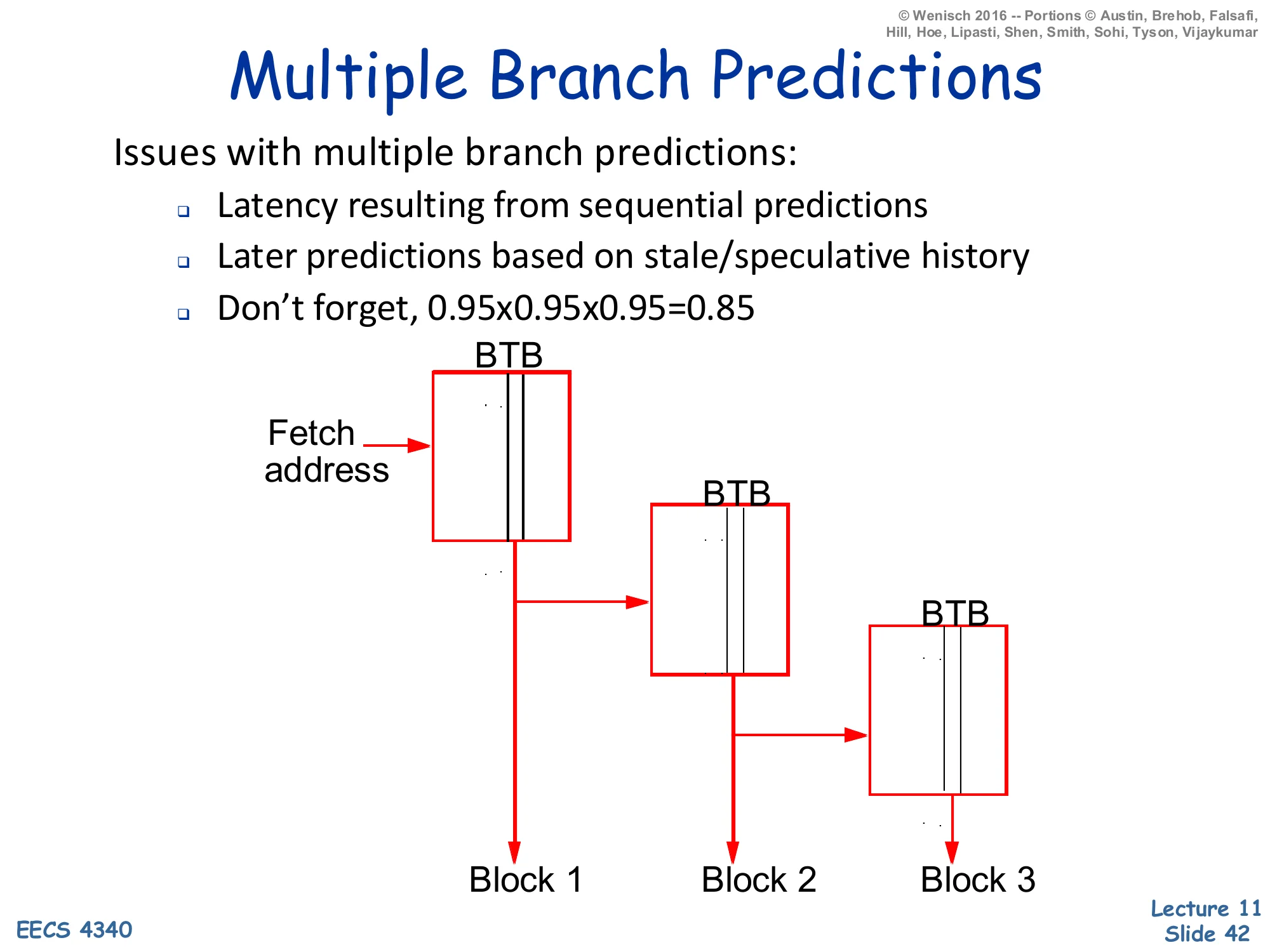
Issues with multiple branch predictions:

• Latency resulting from sequential predictions
• Later predictions based on stale/speculative history
• Don’t forget, $0.95 \times 0.95 \times 0.95 = 0.85$

Diagram: three BTBs chained sequentially — the first BTB takes the fetch address and emits Block 1 and a target, which feeds the second BTB to produce Block 2, which feeds the third BTB to produce Block 3.

Predicting three branches in one cycle by chaining three BTB lookups serialises the latency: the second prediction depends on the first prediction’s target, so the cycle time bloats. Pipelining the predictors helps, but later predictions in the chain run on stale global history (they have not yet seen the outcomes of the earlier branches in the same cycle). Most importantly, the slide reminds the audience of the multiplicative cost of accuracy: 95% per-branch becomes 85% across three branches in one cycle ($0.95^3 \approx 0.857$), meaning that 15% of the time some branch in the wide fetch group is wrong and the entire group has to be re-fetched. So multiple-branch prediction does not just need fast hardware — it needs very accurate per-branch prediction (TAGE-class) just to break even with single-branch prediction at lower fetch widths. The next slides show two algorithms that approximate multiple-branch prediction without the full sequential chain.

Examples of Multi-Branch Predictors — Two-from-One

Slide 43

Show slide text

Examples of Multi-Branch Predictors

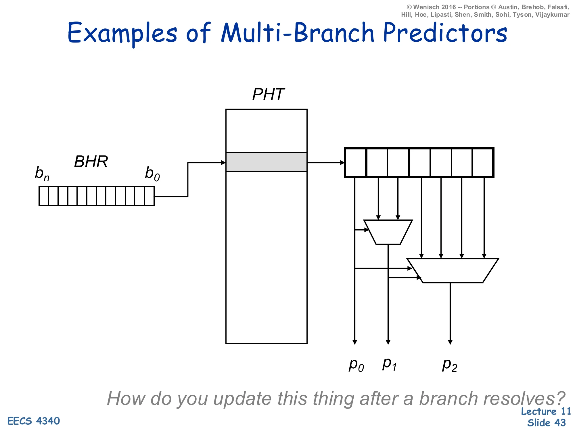
Diagram: BHR (bits $b_n \ldots b_0$) indexes a Pattern History Table; the selected PHT row drives a small lookup that emits three predictions $p_0, p_1, p_2$ via two stacked muxes.

How do you update this thing after a branch resolves?

This is the first multi-branch design: instead of three sequential PHT lookups, the BHR is indexed once and the addressed PHT row holds enough bits to emit several predictions. The first prediction $p_0$ is read directly; the next two are selected by muxes whose select lines are the in-flight predictions themselves (so $p_1$ depends on $p_0$, and $p_2$ depends on both). All three predictions therefore come from the same PHT row, addressed by the same global history, but the position within the row depends on the as-yet-unresolved earlier predictions. The update problem flagged at the bottom of the slide is real: when one of the three branches resolves you have to update the right counter inside the row, and if the resolution flips an earlier prediction you have to repair the predictions that were derived from it. This is the foundation for the Yeh, Marr, Patt design on the next slide.

Examples of Multi-Branch Predictors — Yeh, Marr, Patt

Slide 44

Show slide text

Examples of Multi-Branch Predictors

Diagram (Yeh, Marr, Patt — Figure 3): a Global History Register of width $k$ feeds a PHT of width 2; two wires labelled $k-1$ and $k$ select rows of the PHT. The PHT outputs feed a small mux whose select line decides between the Primary Branch Prediction (using the full $k$-bit history) and a Secondary Branch Prediction (using only $k-1$ history bits, treating the freshly-shifted-in primary prediction as unknown).

Increasing the instruction fetch rate via multiple branch prediction and a branch address cache — https://dl.acm.org/doi/abs/10.1145/165939.165956

Yeh, Marr & Patt’s predictor (HPCA-94) makes two predictions per cycle from a single Global History Register lookup. The trick: the second prediction would depend on the first prediction’s outcome (because that outcome would normally be shifted into the BHR before the second lookup), but the BHR has not yet been updated. So the predictor reads both candidate PHT rows in parallel — the row indexed by BHR ‖ 0 and the row indexed by BHR ‖ 1 — and uses the just-computed primary prediction as the select line of a mux that picks between them. This pays the cost of two PHT reads but eliminates the sequential dependency. The same idea generalises to k branches per cycle by doubling the number of candidate rows for each additional branch — at the cost of $2^{k-1}$ parallel PHT reads. The next slide depicts the multi-port PHT layout that implements this for k = 3.

Examples of Multi-Branch Predictors — 2^(n-2) × 4 PHT

Slide 45

Show slide text

Examples of Multi-Branch Predictors

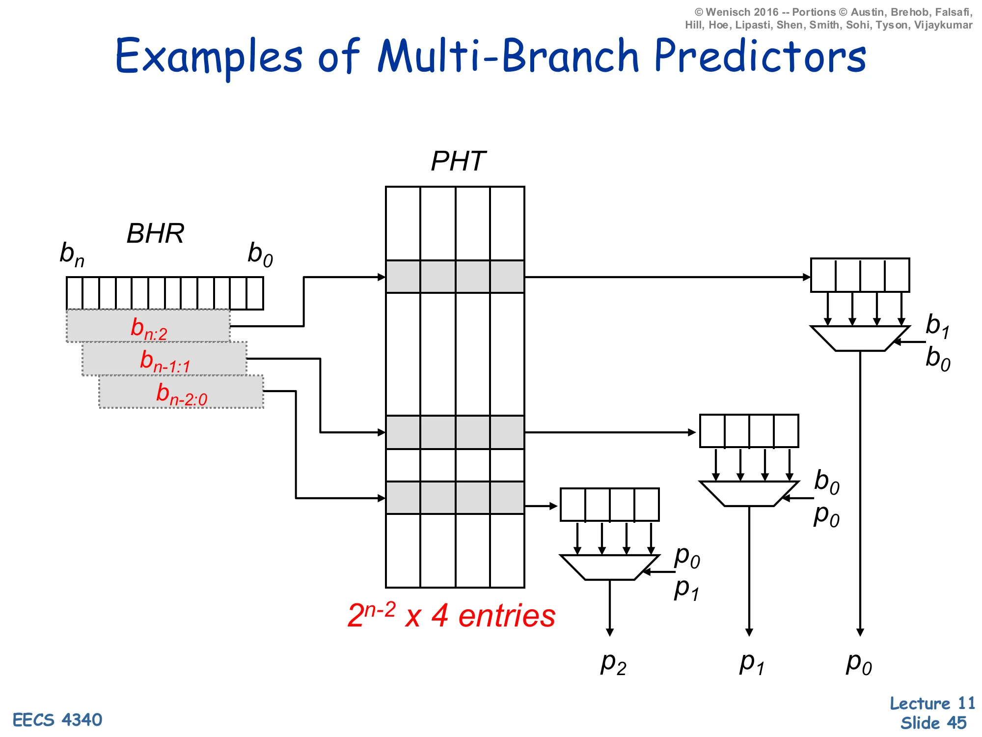
Diagram: BHR (bits $b_n \ldots b_0$). Three overlapping windows of the BHR are highlighted:

• $b_{n:2}$ — the upper bits, used to address the PHT for the first prediction $p_0$
• $b_{n-1:1}$ — shifted by one, used for the second prediction $p_1$
• $b_{n-2:0}$ — shifted by two, used for the third prediction $p_2$

A PHT of $2^{n-2} \times 4$ entries (each entry is 4 saturating counters) is read at three different rows in parallel. Three small 4-input muxes use the predictions and recent BHR bits as select lines:

• $p_0$ row → mux selected by $b_1, b_0$
• $p_1$ row → mux selected by $b_0, p_0$
• $p_2$ row → mux selected by $p_0, p_1$

The three muxes emit $p_2$, $p_1$, $p_0$ in parallel.

This is the full multi-branch predictor implementation: a $2^{n-2} \times 4$ PHT (each row holds 4 counters, indexed by the two least-significant history bits) read at three rows in parallel. The first row is addressed by BHR[n:2] and its 4 counters are demultiplexed by the known low BHR bits b_1, b_0 to produce $p_0$. The second row is addressed by BHR[n-1:1] and its counters are demultiplexed by b_0 and the just-computed $p_0$ to produce $p_1$ (which would have been shifted into bit-0 by the time the second branch’s lookup happened). The third row uses BHR[n-2:0] and is demuxed by $p_0, p_1$ to produce $p_2$. Total cost: 3 parallel SRAM reads plus 3 small muxes. The output rate is one prediction per cycle for each of three branches if the BHR can be shifted by 3 bits per cycle, which is the bottleneck this design replaces.

Multiple Predicted-Taken Branches

Slide 46

Show slide text

Multiple Predicted Taken Branches

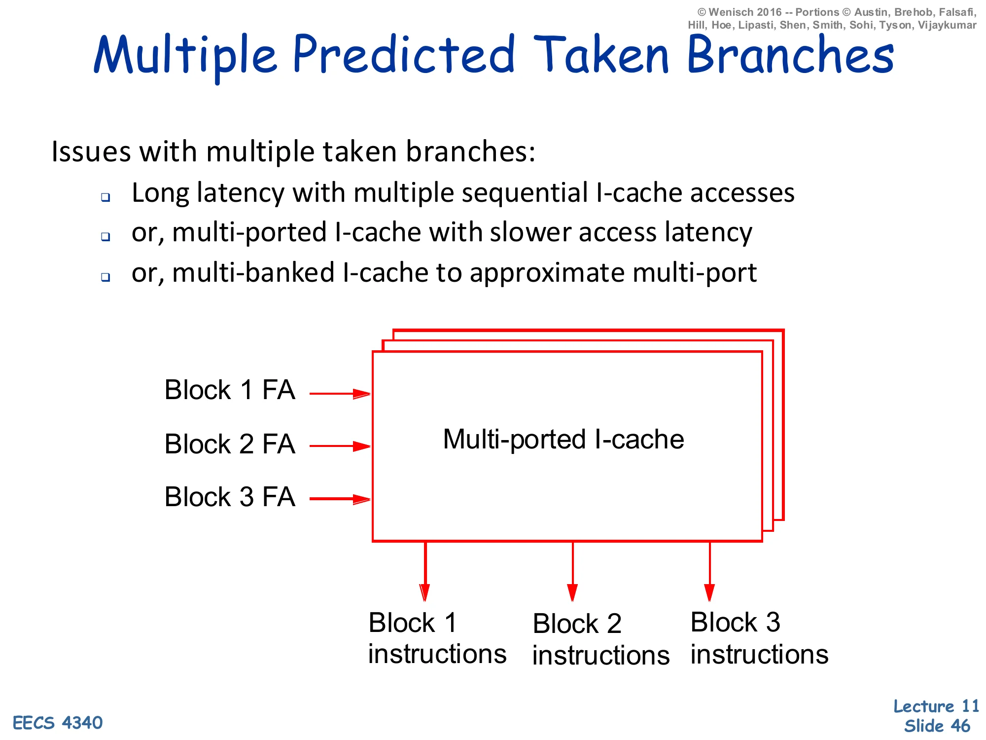
Issues with multiple taken branches:

• Long latency with multiple sequential I-cache accesses
• or, multi-ported I-cache with slower access latency
• or, multi-banked I-cache to approximate multi-port

Diagram: three fetch addresses (Block 1 FA, Block 2 FA, Block 3 FA) feed a multi-ported I-cache that emits Block 1 instructions, Block 2 instructions, and Block 3 instructions in parallel.

Even with multiple branch predictions in hand, the I-cache still has to deliver instructions from each predicted-taken target in the same cycle. Three options exist, each with a cost. (1) Sequential lookups: cheapest in area, but latency adds up — three lookups at one cycle each is a 3-cycle bubble. (2) True multi-ported I-cache: every port can read independently, but multi-porting an SRAM costs roughly N² in area for N ports and slows the cycle time. (3) Multi-banked I-cache: cheaper than true multi-port — the cache is sliced into independent SRAM banks and each port reads from a different bank — but bank conflicts (two predicted-taken branches whose targets happen to live in the same bank) cause stalls. The next slide adds the alignment-and-collapsing problem on top of all this, and slide 48 shows that a trace cache subsumes both.

Instruction Alignment and Collapsing

Slide 47

Show slide text

Instruction Alignment and Collapsing

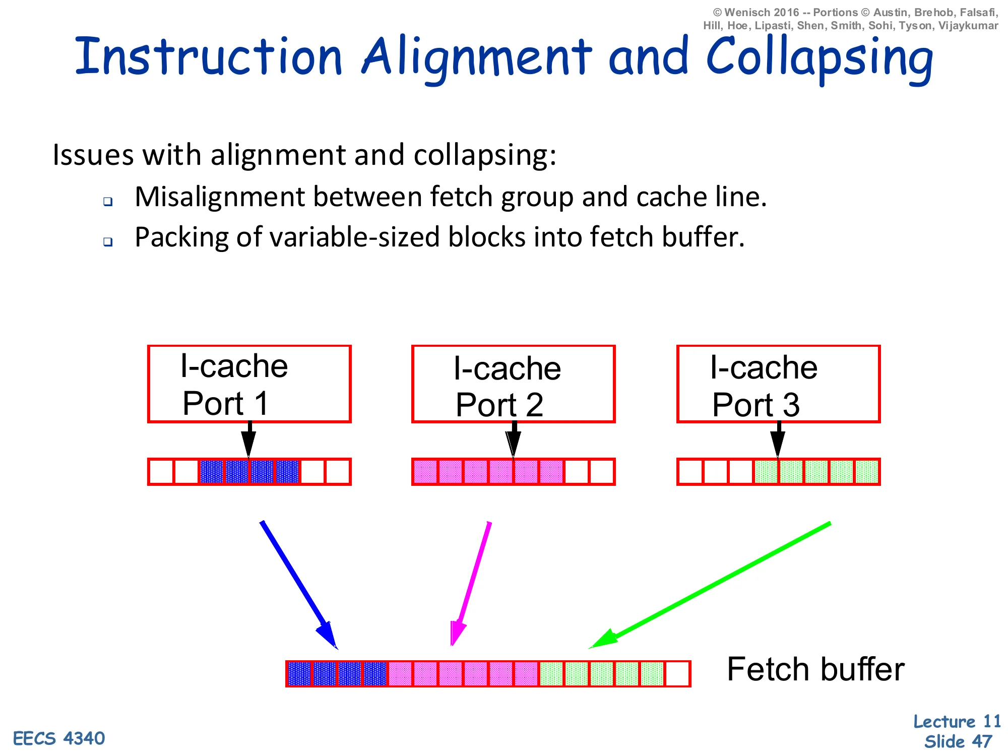
Issues with alignment and collapsing:

• Misalignment between fetch group and cache line.
• Packing of variable-sized blocks into fetch buffer.

Diagram: three I-cache ports each return a partial cache line containing some useful instructions (highlighted in different colours) at arbitrary offsets within the line. A combining/collapsing network packs the highlighted bytes from all three ports into a contiguous fetch buffer.

Even when the I-cache delivers three blocks in parallel, the useful instructions inside each block are a sub-window — the trailing portion of the block containing the entry point of the next basic block, and the leading portion ending at the next predicted-taken branch. So the front end has to extract those sub-windows from each port and pack them contiguously into the fetch buffer for decode. This “collapsing network” is essentially a configurable byte-shifter and merger; it is wide (one bit per byte position per port) and slow. The slide’s diagram makes the size of the wiring clear: three ports, each returning a full cache line, all feed into a single bit-level multiplexer that has to produce one ordered sequence of instructions. Combined with multi-ported lookup, multi-branch prediction, and recovery, the front end of an 8-wide processor becomes one of the most complex parts of the chip — which is the motivation for trace caches.

Trace Cache Motivation

Slide 48

Show slide text

Trace Cache Motivation

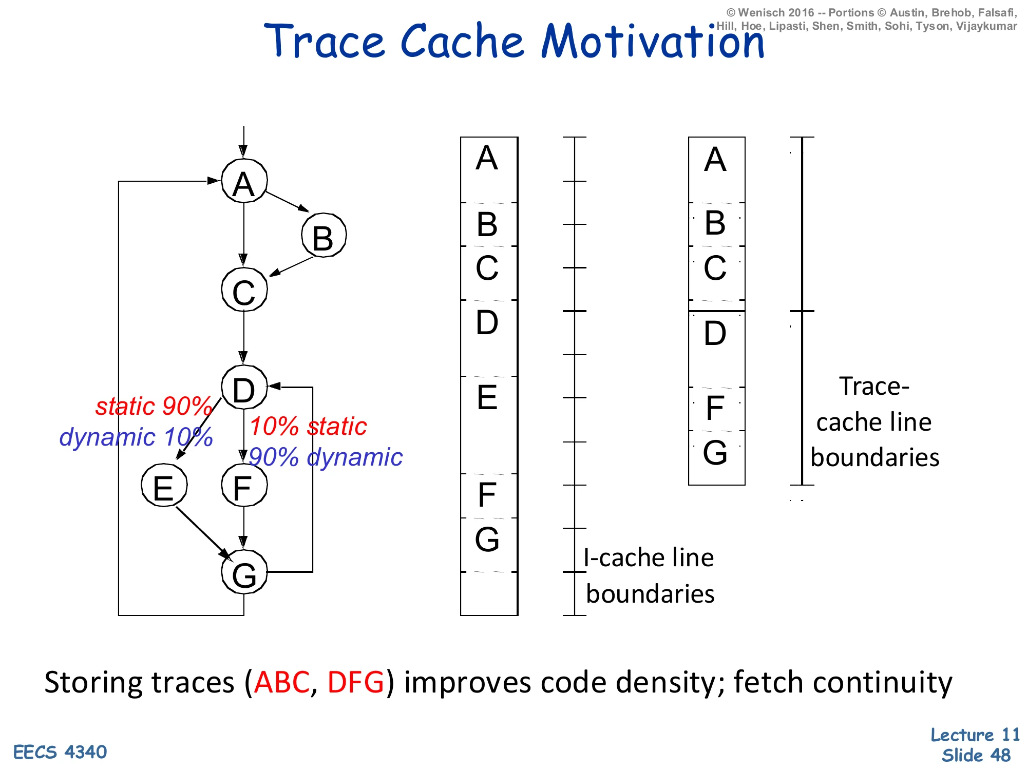
Left: a control-flow graph with basic blocks A → B → C → D → {E (10% dynamic), F (90% dynamic)} → G. The edge A→B is annotated static 90%, dynamic 10% and the edge D→F is annotated 10% static, 90% dynamic.

Middle: a traditional I-cache layout with cache-line boundaries cutting across blocks A, B, C, D, E, F, G stored in static program order.

Right: a trace-cache layout where the dominant dynamic trace A, B, C, D, F, G is stored as one contiguous trace, with trace-cache-line boundaries cutting across the trace.

Storing traces (ABC, DFG) improves code density; fetch continuity

In the example CFG, block A’s fall-through to B happens 90% statically (in the source) but only 10% dynamically (at runtime); the back-edge D→F is rare statically but dominant dynamically. A traditional I-cache stores instructions in static program order, so the dynamic trace A,B,C,D,F,G is scattered across multiple cache lines and requires the multi-bank, multi-port, alignment-and-collapsing machinery from the previous slides to fetch in one cycle. A trace cache instead caches the dynamic trace itself: the line A,B,C,D,F,G is stored contiguously and is delivered in one access. Block E (10% dynamic) lives in the regular I-cache as a fall-back. Trace caches make wide fetch dramatically simpler — but they introduce duplication (the same static block can appear in many different traces) and consistency issues on self-modifying code, and they need their own predictor to predict the next trace rather than the next branch (slide 49).

Trace Cache

Slide 49

Show slide text

Trace Cache

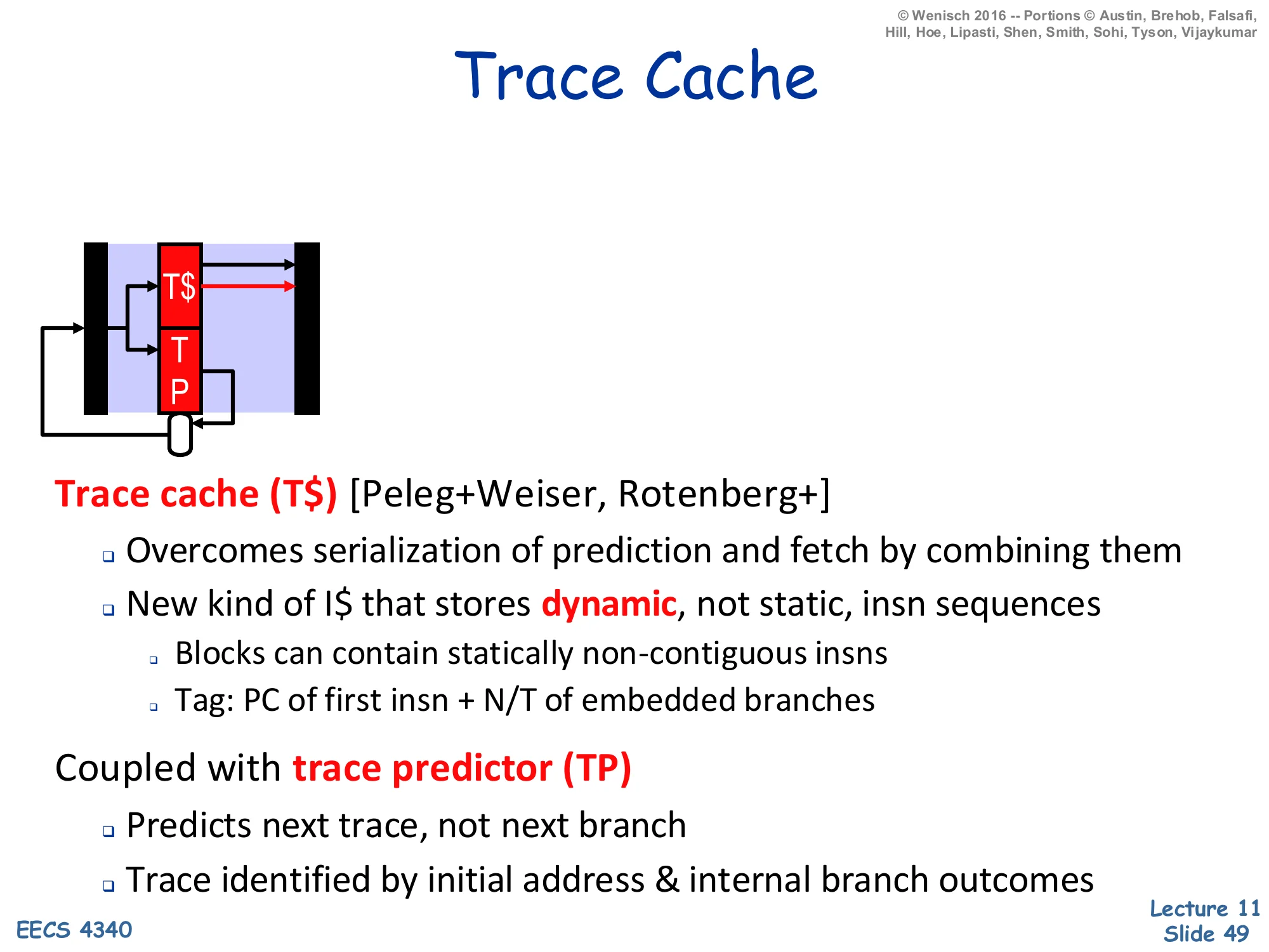
Diagram: front-end pipeline icon with a Trace Cache (T$) sitting in the fetch position normally occupied by the I$, plus a dedicated Trace Predictor (TP) that loops back to T$.

Trace cache (T$) [Peleg+Weiser, Rotenberg+]

• Overcomes serialization of prediction and fetch by combining them
• New kind of I$ that stores dynamic, not static, insn sequences
  • Blocks can contain statically non-contiguous insns
  • Tag: PC of first insn + N/T of embedded branches

Coupled with trace predictor (TP)

• Predicts next trace, not next branch
• Trace identified by initial address & internal branch outcomes

The trace cache is jointly the work of Peleg & Weiser (Intel) and Rotenberg, Bennett & Smith (Wisconsin). The structural change is that the storage unit is a dynamic trace, not a static cache line: a trace might contain blocks A,B,C,D,F,G stored contiguously even though F lives at a non-adjacent static PC. The tag is a composite of the PC of the first instruction in the trace plus the taken/not-taken pattern of every branch embedded inside the trace — different control-flow paths through the same starting PC become different trace-cache entries. Fetch is a single SRAM read followed by no alignment/collapsing, because the trace is already contiguous. To take advantage of this layout the front end needs a trace predictor that predicts the next trace (an entire control-flow path) rather than the next individual branch. Trace predictors typically use a longer global-history hash than direction predictors do, because predicting a multi-block path is fundamentally harder than predicting a single binary outcome.

Trace Cache Example

Slide 50

Show slide text

Trace Cache Example

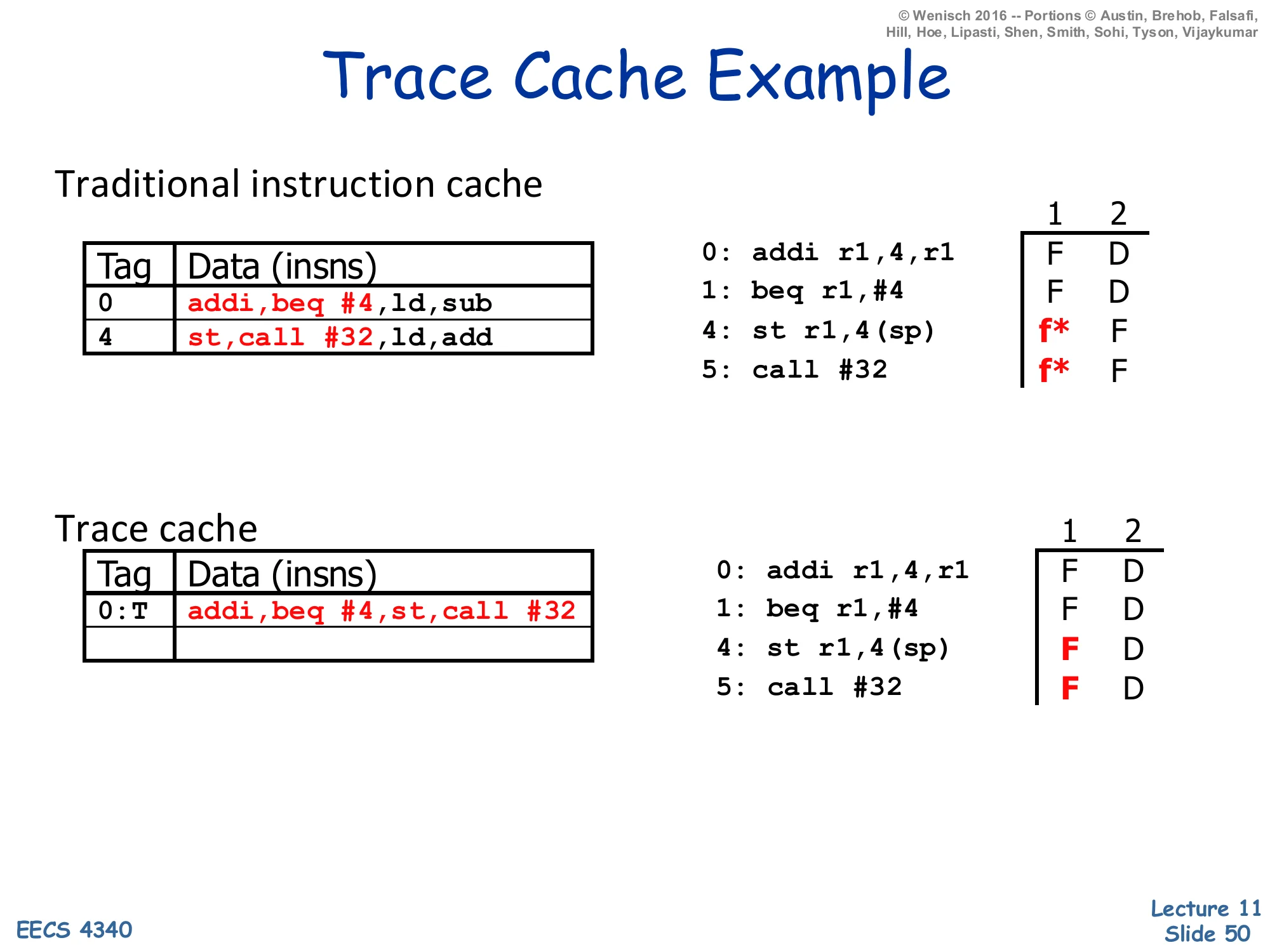
Traditional instruction cache

Tag	Data (insns)
0	addi, beq #4, ld, sub
4	st, call #32, ld, add

Dynamic schedule:

0: addi r1,4,r1   F  D
1: beq  r1,#4     F  D
4: st   r1,4(sp)  f* F
5: call #32       f* F

(f* = fetch slot wasted because a taken branch redirects fetch to a different cache line.)

Trace cache

Tag	Data (insns)
0:T	addi, beq #4, st, call #32

Dynamic schedule:

0: addi r1,4,r1   F  D
1: beq  r1,#4     F  D
4: st   r1,4(sp)  F  D
5: call #32       F  D

The example shows a 4-instruction window starting at PC 0: addi; beq #4; ld; sub, where the beq #4 branch is predicted-taken with target PC 4, where st; call #32; ld; add lives. With a traditional I-cache (top), one fetch reads the line starting at PC 0 and gets addi, beq, ld, sub — but only addi and beq are useful because the branch is taken. The next cycle has to read a different cache line at PC 4 to get st, call, so two of the four would-be-fetched slots (f*) are wasted. With a trace cache (bottom), the dynamic trace addi, beq, st, call #32 is stored contiguously under tag 0:T (the colon-T encodes the predicted Taken outcome of the branch inside the trace). One fetch returns four useful instructions, all of which proceed straight to decode. The dynamic schedule on the right shows the same four instructions flowing into Decode without any wasted slots — exactly the wide-fetch property the lecture has been chasing.

Readings

Slide 51

Show slide text

Readings

For today:

• H & P Chapter 3.9
• McFarling: Combining Branch Predictors
• Increasing the instruction fetch rate via multiple branch prediction and a branch address cache, https://dl.acm.org/doi/abs/10.1145/165939.165956
• Trace cache: a low latency approach to high bandwidth instruction fetching, https://ieeexplore.ieee.org/abstract/document/566447

The readings slide is repeated at the end of the deck as a reminder. H&P Chapter 3.9 covers the textbook material on dynamic branch prediction (BHT, BTB, correlated, tournament). McFarling’s paper introduces gshare and the hybrid/tournament predictor used by the Alpha 21264 — material covered on slides 28–29. Yeh, Marr & Patt’s Increasing the instruction fetch rate paper is the source of the multi-branch-prediction material on slides 42–45. Rotenberg, Bennett & Smith’s Trace cache paper is the source of the trace-cache material on slides 48–50. The deck is essentially a guided tour of these four sources, and reading them gives the prerequisite vocabulary (gshare, tournament, BAC, trace, fill unit) that recurs in every modern branch-prediction paper.

Announcements

Slide 52

Show slide text

Announcements

Project #4

• Due: milestone 3, 8-April-26
• In-person mandatory project check-in
  • 8:40–8:50 AM: CCDYMP
  • 8:50–9:00 AM: G13
  • 9:00–9:10 AM: GaPiChiXuXu
  • 9:10–9:20 AM: OoO
  • 9:20–9:30 AM: RISCy Whisky
  • 9:30–9:40 AM: SIX
  • 9:40–9:50 AM: UNI

Optional project meetings

• Mondays and Wednesdays during my office hours

https://courseworks2.columbia.edu/courses/237081