L09 · Memory Scheduling
Topic: out-of-order · 50 pages
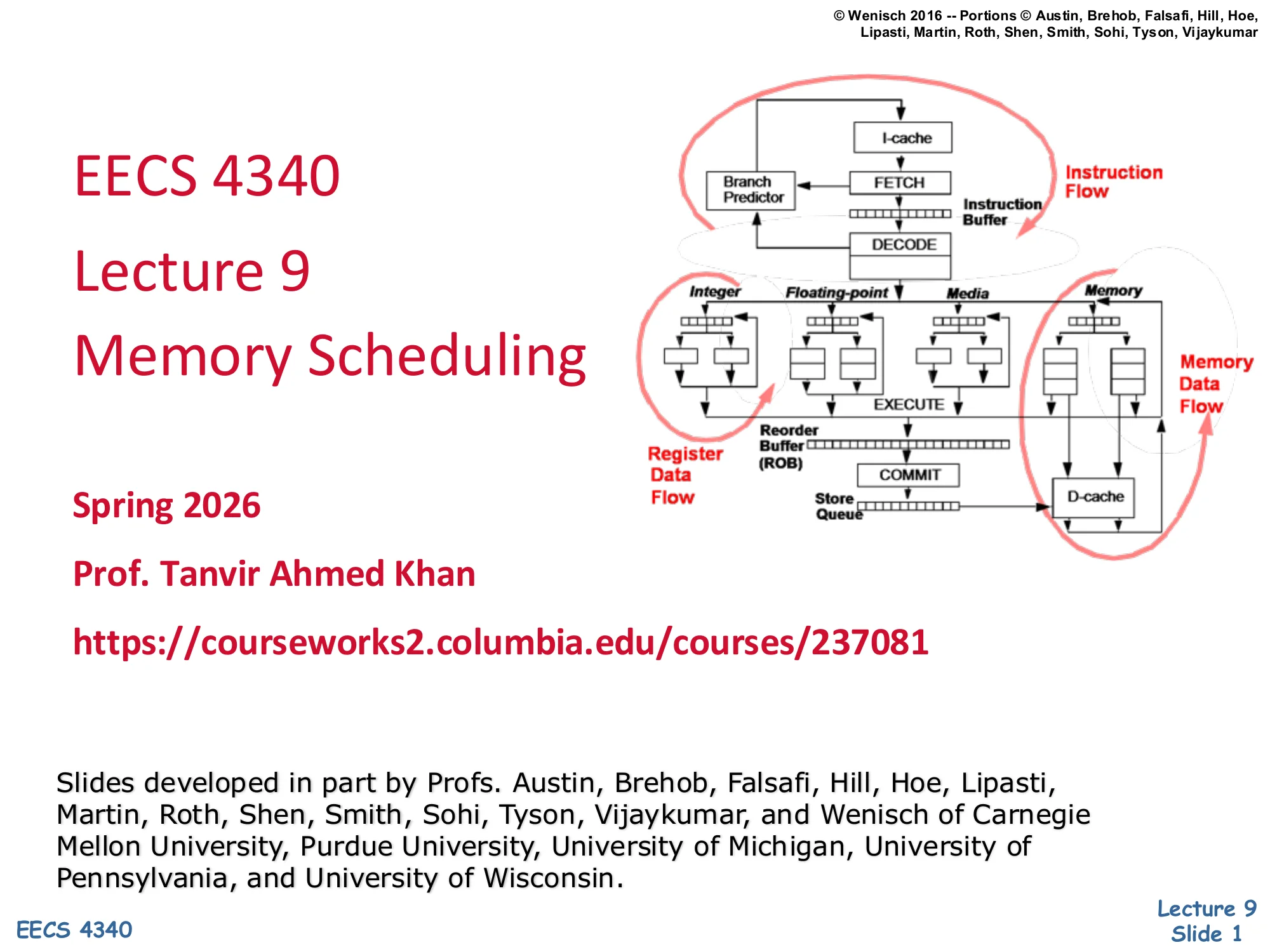
EECS 4340 Lecture 9 — Memory Scheduling
Announcements

Show slide text
Announcements
- Project #4
- Due: milestone 3, 8-Apr-26
- Project meetings
- Mondays and Wednesdays during my office hours
- Mondays: CCDYMP, G13, GaPiChiXuXu, OoO
- Wednesdays: RISCy Whisky, SIX, UNI
- Mondays and Wednesdays during my office hours
Recap: MIPS R10K Microarchitecture
MIPS R10K: Alternative Implementation
Show slide text
MIPS R10K: Alternative Implementation
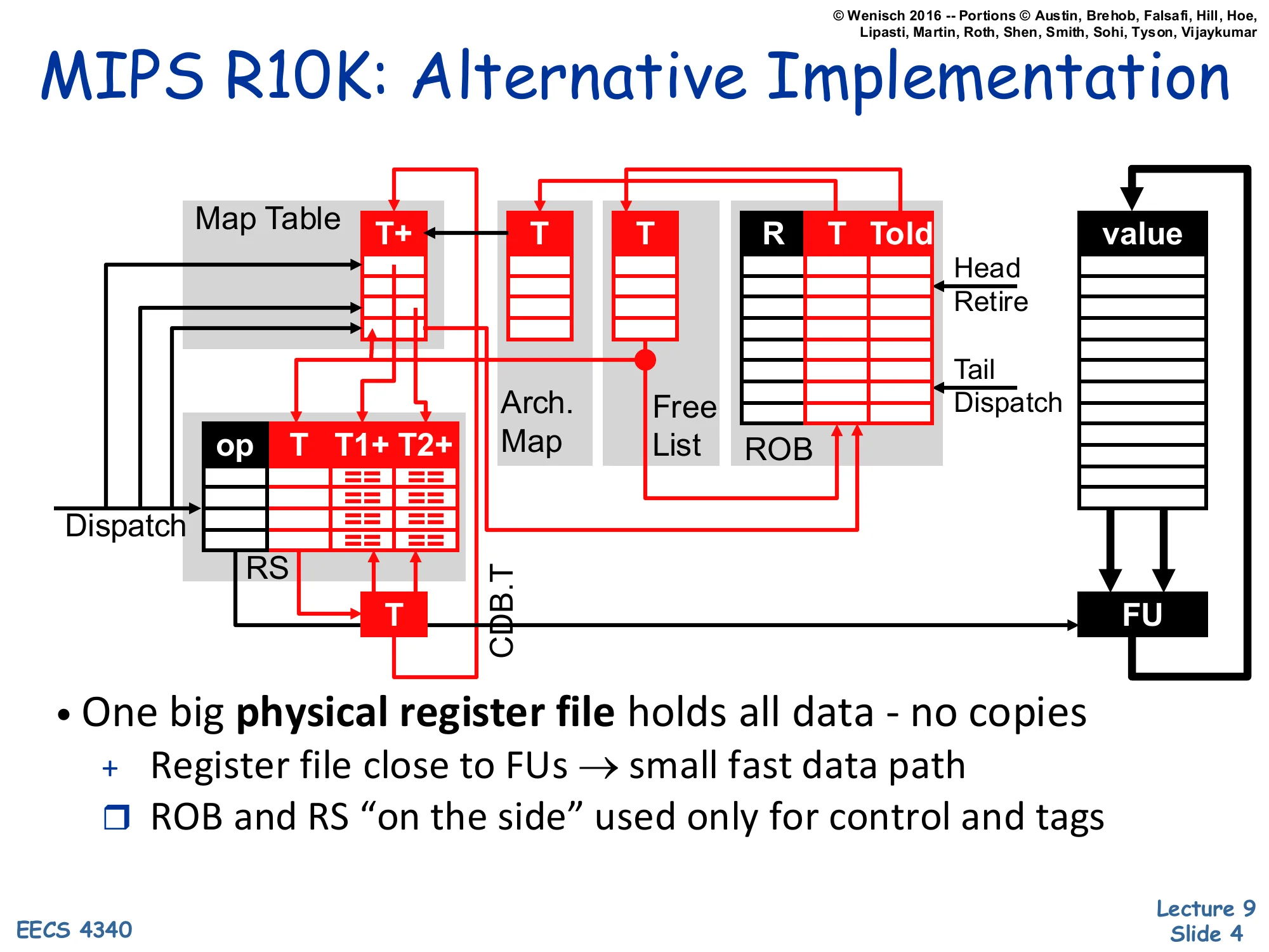
Dispatch path: Map Table (T+) feeds an op | T | T1+ | T2+ field, an Arch. Map, and a Free List that supplies physical register numbers. Output T fans into the ROB (Head=Retire, Tail=Dispatch) holding T | Told | value.
Reservation Stations match incoming CDB.T tags against waiting == comparators, then dispatch a tag T to a Functional Unit (FU).
- One big physical register file holds all data — no copies
- Register file close to FUs → small fast data path
- ROB and RS “on the side” used only for control and tags
This recap slide reintroduces the MIPS R10K out-of-order organization that L08 covered. Unlike P6 (where each in-flight value lives in some combination of the architectural register file, the ROB, and the reservation station), R10K keeps every value in one large physical register file (PRF) sitting next to the functional units. The Map Table (T+) tracks the current physical-register name for each architectural register and a ready bit. A Free List supplies fresh physical-register names at dispatch, and the ROB tracks both the new name (T) and the previous one (Told) so that on commit the Told entry can be returned to the free list. Reservation stations only carry tags T1+, T2+, not values — when a result broadcasts on the CDB, waiting RS entries match the tag and become ready. The headline benefit is short, fast data paths: results never have to traverse the wide ROB or RS — they go FU → PRF → FU, which is what made R10K-style designs scale to higher frequencies in the late 1990s.
Register Renaming in R10K
Show slide text
Register Renaming in R10K
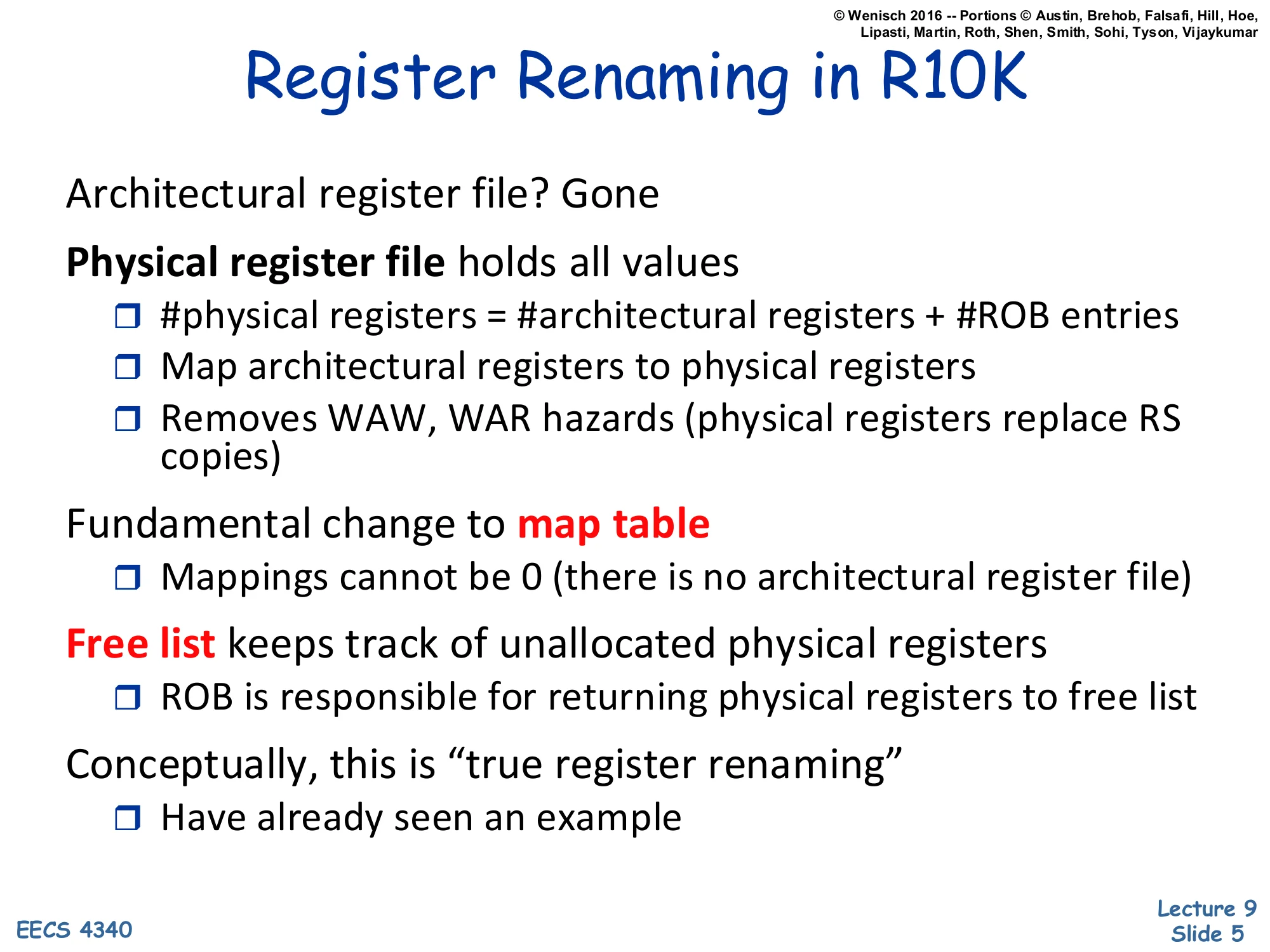
- Architectural register file? Gone
- Physical register file holds all values
- #physical registers = #architectural registers + #ROB entries
- Map architectural registers to physical registers
- Removes WAW, WAR hazards (physical registers replace RS copies)
- Fundamental change to map table
- Mappings cannot be 0 (there is no architectural register file)
- Free list keeps track of unallocated physical registers
- ROB is responsible for returning physical registers to free list
- Conceptually, this is “true register renaming”
- Have already seen an example
R10K implements true register renaming: there is no separate architectural register file, only one PRF that is large enough to hold every architectural register plus every in-flight ROB entry. Every architectural register name is always mapped to exactly one physical register; the Map Table never holds a null mapping. Because each new write allocates a fresh physical register from the free list, WAW and WAR hazards disappear by construction — no two in-flight writes can collide on the same physical name. The ROB’s job in R10K is no longer to hold values but to free physical registers in order: at commit, the Told entry of the retiring instruction is the previous physical mapping for that architectural register and is now safe to return to the free list, since no younger instruction can need it. The slide labels this “true” renaming to contrast with P6’s copy-based scheme, where rename happens implicitly via ROB-to-ARF copying at commit.
R10K Data Structures
Show slide text
R10K Data Structures
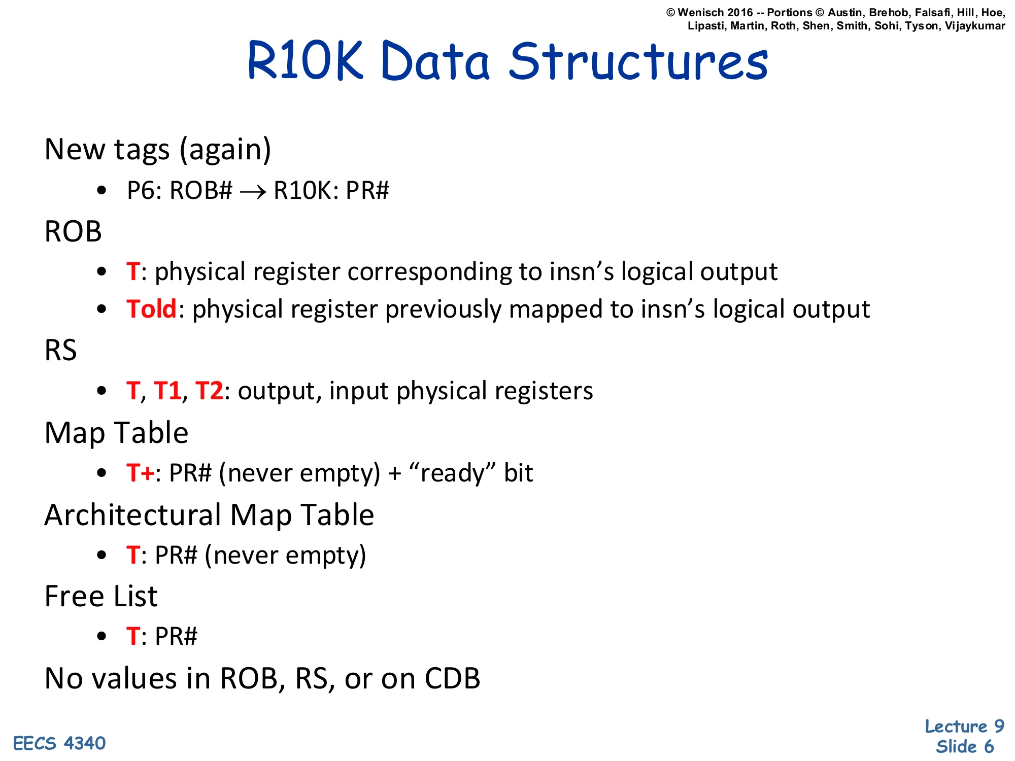
- New tags (again)
- P6: ROB# → R10K: PR#
- ROB
- T: physical register corresponding to insn’s logical output
- Told: physical register previously mapped to insn’s logical output
- RS
- T, T1, T2: output, input physical registers
- Map Table
- T+: PR# (never empty) + “ready” bit
- Architectural Map Table
- T: PR# (never empty)
- Free List
- T: PR#
- No values in ROB, RS, or on CDB
The bookkeeping change from P6 to R10K is subtle but consequential. The dataflow tag is no longer the ROB index — it is a physical-register number (PR#), so every consumer waits on a PR# rather than a slot. Each ROB entry stores both T (the new mapping for this instruction’s destination architectural register) and Told (whatever PR# used to be mapped). The Map Table holds the current (speculative) mapping plus a ready bit; the Architectural Map Table holds the committed mapping and is updated only at retire. The free list holds PR#s currently not mapped anywhere. The crucial line — “No values in ROB, RS, or on CDB” — captures the entire architectural philosophy: the CDB broadcasts only tags, results land directly in the PRF, and the data path between functional units stays narrow. Compare to P6, where the ROB carries 64-bit (or wider) values for every entry and the CDB ferries data.
R10K Data Structures — Initial State
Show slide text
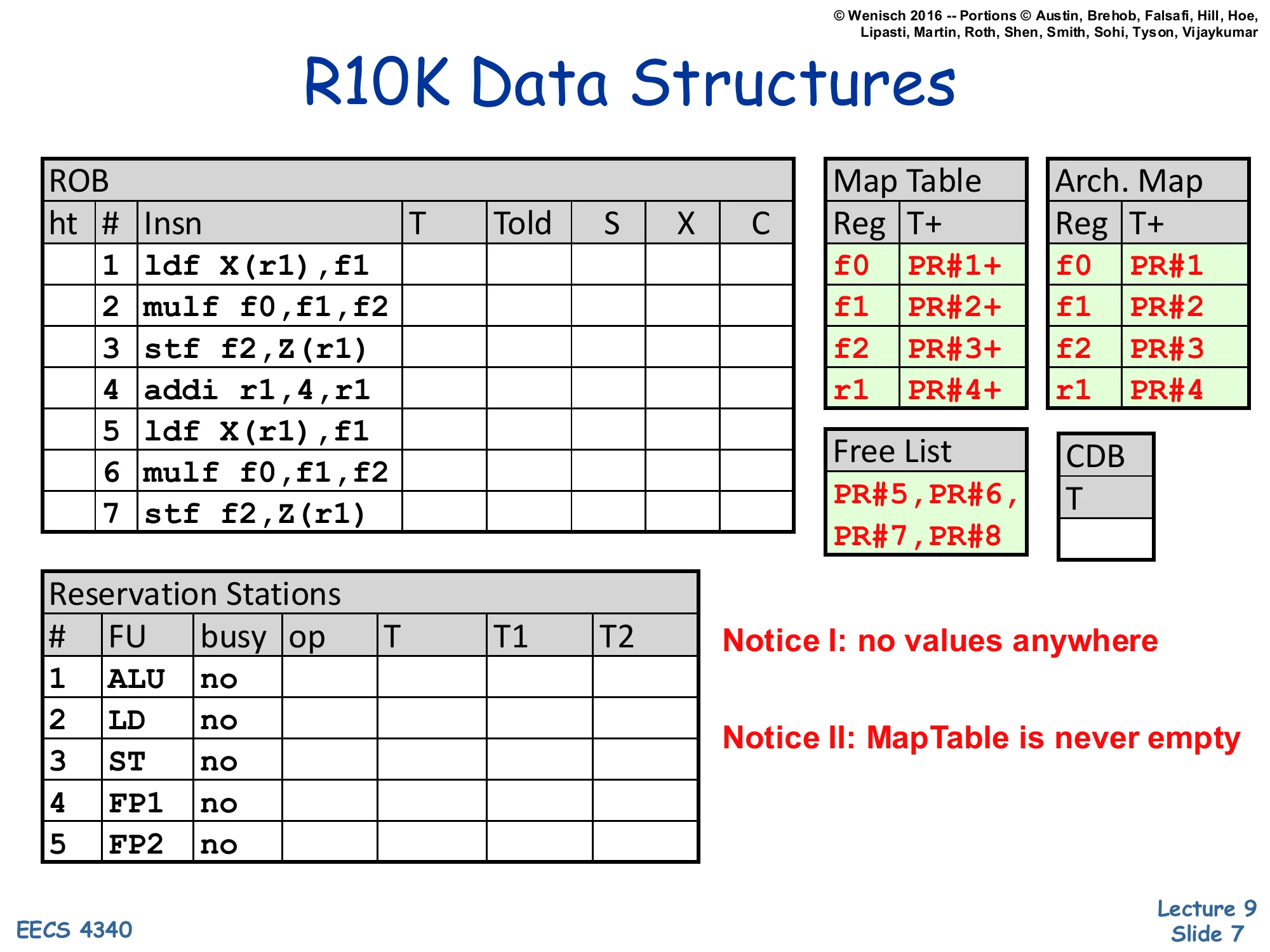
R10K Data Structures
ROB
| ht | # | Insn | T | Told | S | X | C |
|---|---|---|---|---|---|---|---|
| 1 | ldf X(r1),f1 | ||||||
| 2 | mulf f0,f1,f2 | ||||||
| 3 | stf f2,Z(r1) | ||||||
| 4 | addi r1,4,r1 | ||||||
| 5 | ldf X(r1),f1 | ||||||
| 6 | mulf f0,f1,f2 | ||||||
| 7 | stf f2,Z(r1) |
Map Table: f0→PR#1+, f1→PR#2+, f2→PR#3+, r1→PR#4+
Arch. Map: f0→PR#1, f1→PR#2, f2→PR#3, r1→PR#4
Free List: PR#5, PR#6, PR#7, PR#8
Reservation Stations: 5 entries (ALU, LD, ST, FP1, FP2), all busy=no.
CDB: T (idle).
Notice I: no values anywhere. Notice II: MapTable is never empty.
This is the starting tableau for the worked example that runs through the recap. Seven instructions are queued in the ROB (the same loop body that L08 used: a load, a multiply, a store, a pointer increment, then the same three again). The Map Table maps the four logical registers (f0, f1, f2, r1) to PR#1–PR#4 with their + ready bits set, since these values came from before the trace. The Free List has four spare physical registers (PR#5–PR#8) ready for renaming. The two annotations on the slide are the headline takeaways: there are no data values stored anywhere in this snapshot — only PR# tags — and the Map Table never has a null entry, so any reader can always locate the current physical register holding any architectural value. The reservation stations and CDB are idle because dispatch hasn’t yet started.
P6 vs. R10K (Renaming)
Show slide text
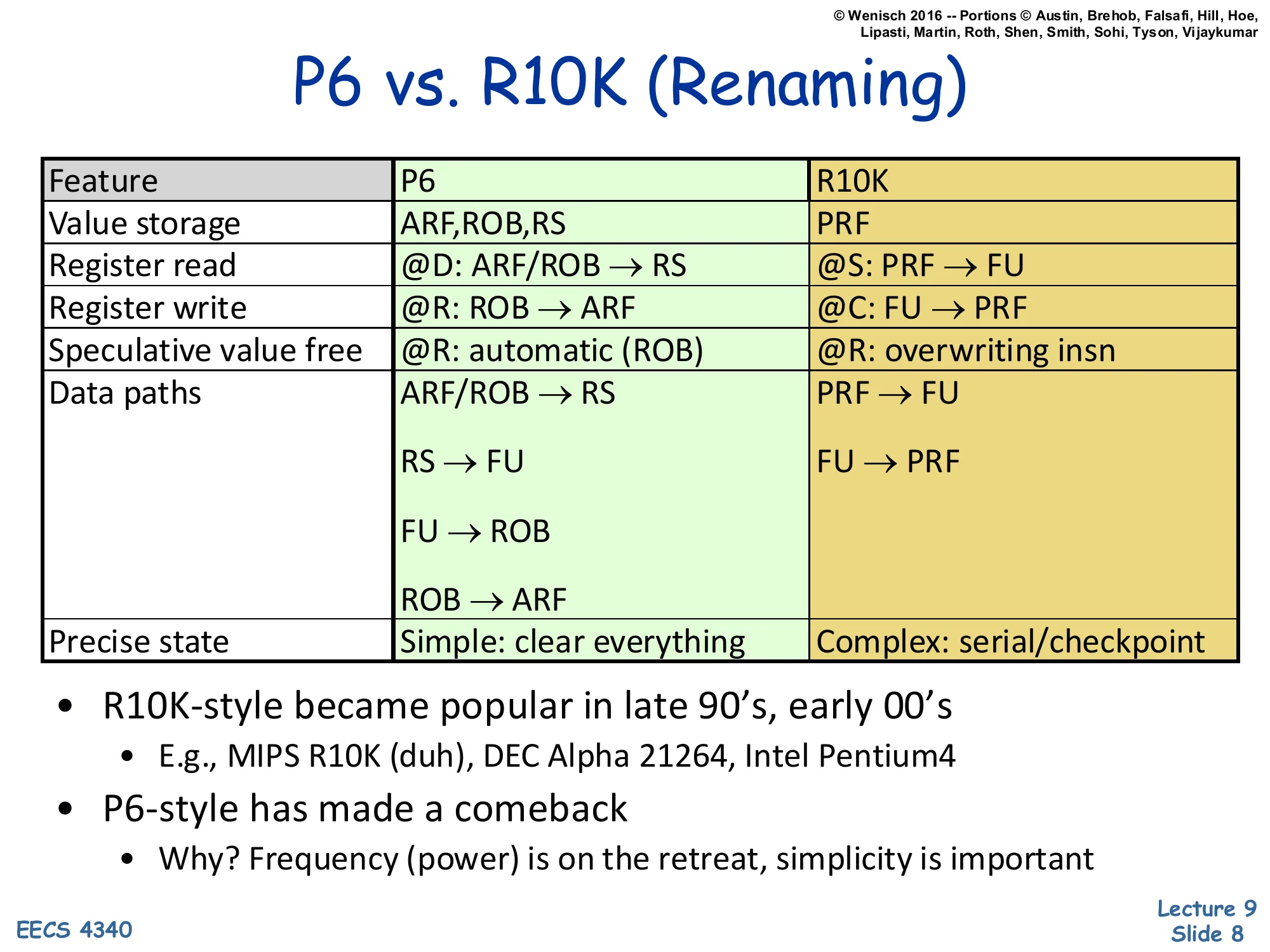
P6 vs. R10K (Renaming)
| Feature | P6 | R10K |
|---|---|---|
| Value storage | ARF, ROB, RS | PRF |
| Register read | @D: ARF/ROB → RS | @S: PRF → FU |
| Register write | @R: ROB → ARF | @C: FU → PRF |
| Speculative value free | @R: automatic (ROB) | @R: overwriting insn |
| Data paths | ARF/ROB → RS; RS → FU; FU → ROB; ROB → ARF | PRF → FU; FU → PRF |
| Precise state | Simple: clear everything | Complex: serial/checkpoint |
- R10K-style became popular in late 90’s, early 00’s
- E.g., MIPS R10K (duh), DEC Alpha 21264, Intel Pentium4
- P6-style has made a comeback
- Why? Frequency (power) is on the retreat, simplicity is important
This table is the cleanest summary of the P6-vs-R10K trade. In P6, an in-flight value can live in three places (ARF, ROB, or RS) and registers are read at Dispatch — RS entries actually carry copies of operand values. In R10K, every value lives in the PRF and is read at Schedule time, just before issue, so the RS only stores tags. P6’s commit step copies a value from the ROB into the ARF; R10K’s commit step is just a pointer swap in the Architectural Map Table. The two designs trade off precise-state recovery: P6’s recovery is trivially “clear all speculative state” because the ARF still holds the committed values, while R10K must walk back the Map Table — either serially via the ROB or by restoring a checkpoint. The closing bullet notes that R10K-style won the late-1990s frequency race (Alpha 21264, Pentium 4) but P6-style has returned because modern designs prize energy efficiency and design simplicity over peak clock.
Summary (Renaming)
Show slide text
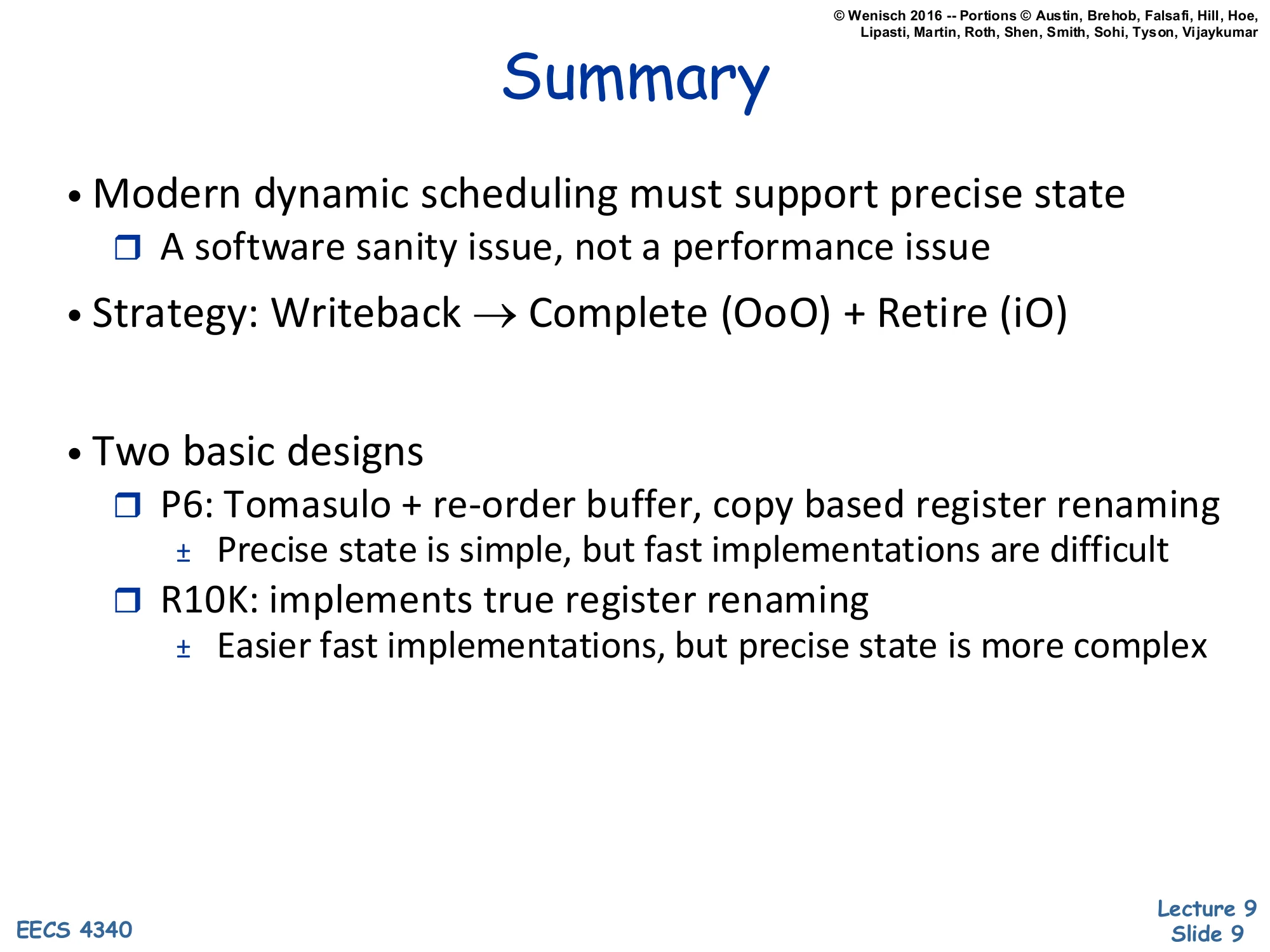
Summary
-
Modern dynamic scheduling must support precise state
- A software sanity issue, not a performance issue
-
Strategy: Writeback → Complete (OoO) + Retire (iO)
-
Two basic designs
- P6: Tomasulo + re-order buffer, copy based register renaming
- ± Precise state is simple, but fast implementations are difficult
- R10K: implements true register renaming
- ± Easier fast implementations, but precise state is more complex
- P6: Tomasulo + re-order buffer, copy based register renaming
This wrap-up of the renaming material crystallizes the rule: dynamic scheduling can run instructions out of order, but commits must look in-order to preserve precise state for software. Both major designs split writeback (which would update architectural state in P6 or PRF in R10K) from retire (which is in-order and may be many cycles later). Tomasulo supplied the OoO-execution machinery; the reorder buffer supplied the precise-state machinery; combining them is the P6 design. R10K replaced P6’s value-carrying ROB with a unified PRF and explicit register renaming. The ± marks emphasize the symmetric trade: P6 is simple to make precise but hard to make fast; R10K is easy to make fast but hard to recover precisely. With this recap done, the lecture pivots to the missing piece: how to schedule loads and stores out of order, where neither algorithm yet handles memory-address dependences.
Dynamic Scheduling Summary
Show slide text
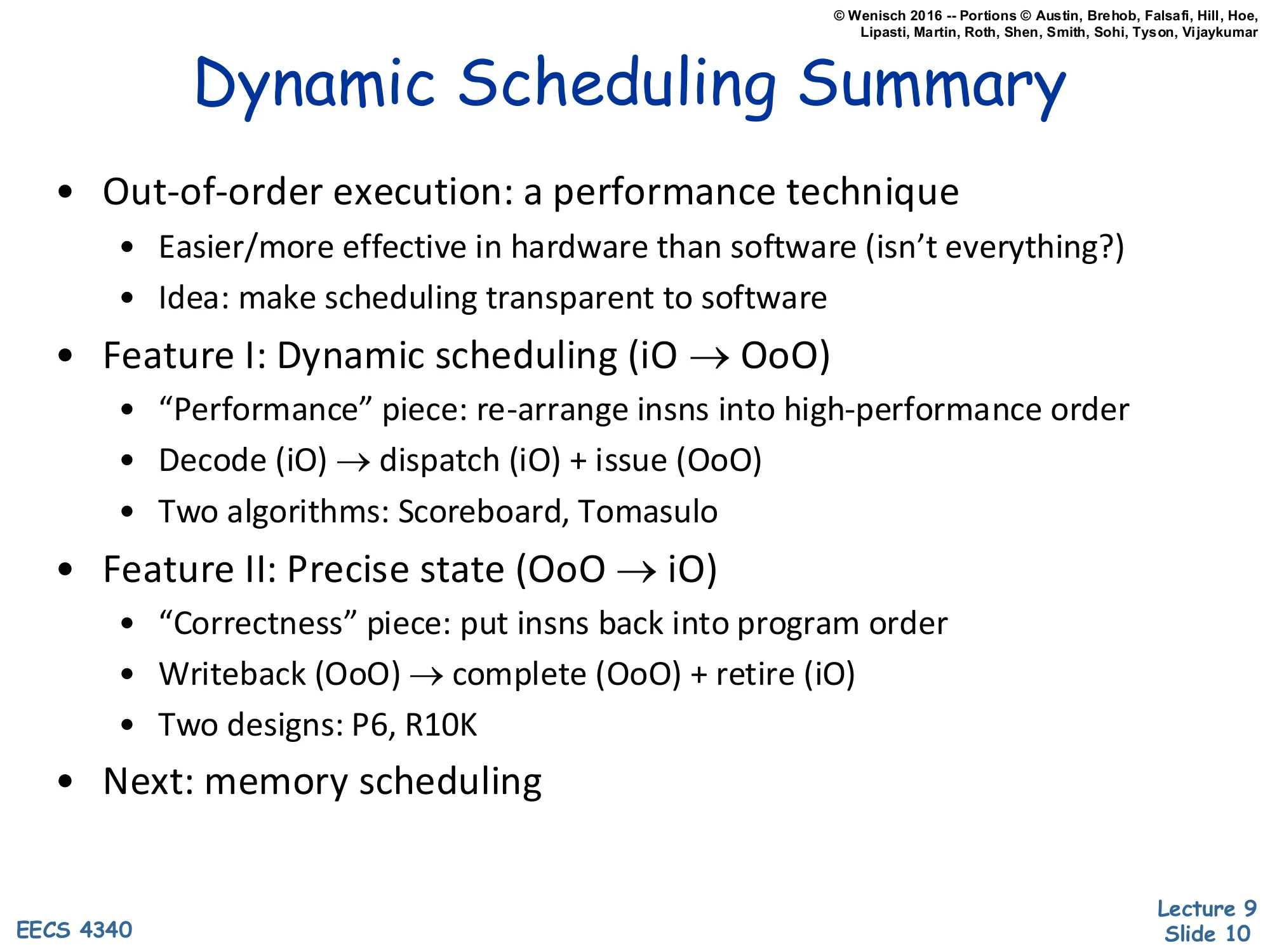
Dynamic Scheduling Summary
- Out-of-order execution: a performance technique
- Easier/more effective in hardware than software (isn’t everything?)
- Idea: make scheduling transparent to software
- Feature I: Dynamic scheduling (iO → OoO)
- “Performance” piece: re-arrange insns into high-performance order
- Decode (iO) → dispatch (iO) + issue (OoO)
- Two algorithms: Scoreboard, Tomasulo
- Feature II: Precise state (OoO → iO)
- “Correctness” piece: put insns back into program order
- Writeback (OoO) → complete (OoO) + retire (iO)
- Two designs: P6, R10K
- Next: memory scheduling
The two-feature view is the cleanest mental model for OoO execution. Feature I is the performance feature: the front end decodes and dispatches in program order, but the issue logic (scoreboarding or Tomasulo) reorders instructions to start whichever ones have ready operands. Feature II is the correctness feature: even though instructions complete out of order, the retire stage walks the ROB in program order so that architectural state updates remain in-order, preserving precise interrupts. The remaining gap — and the topic of the rest of L09 — is that neither feature, as presented, handles memory dependences. Register renaming makes register dependences trivial because the names are statically known at decode; memory addresses are not known at decode, so the same machinery cannot tell whether a younger load depends on an older store. The next slides build the load/store queues that fix this.
Memory Scheduling
Out of Order Memory Operations
Show slide text
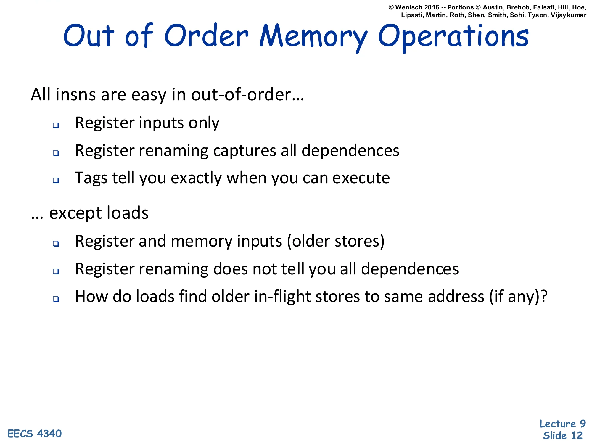
Out of Order Memory Operations
- All insns are easy in out-of-order…
- Register inputs only
- Register renaming captures all dependences
- Tags tell you exactly when you can execute
- … except loads
- Register and memory inputs (older stores)
- Register renaming does not tell you all dependences
- How do loads find older in-flight stores to same address (if any)?
This is the slide that motivates the entire lecture. For an arithmetic instruction, every input is a register name fixed at decode, so register renaming turns the dependence graph into a clean DAG and tag matching delivers operands the moment they’re produced. Loads break this model: a load reads from memory, and the most recent producer of that memory location may be an older in-flight store whose address is not yet known at the time the load wants to issue. The hardware cannot decide whether the load has a RAW dependence on a particular store until both addresses have been computed. This forces a new structure — the load/store queue — that plays the same role for memory that the renaming map plays for registers, plus a new technique — memory disambiguation — for deciding when an unknown-address store can be safely bypassed.
Dynamic Reordering of Memory Operations
Show slide text
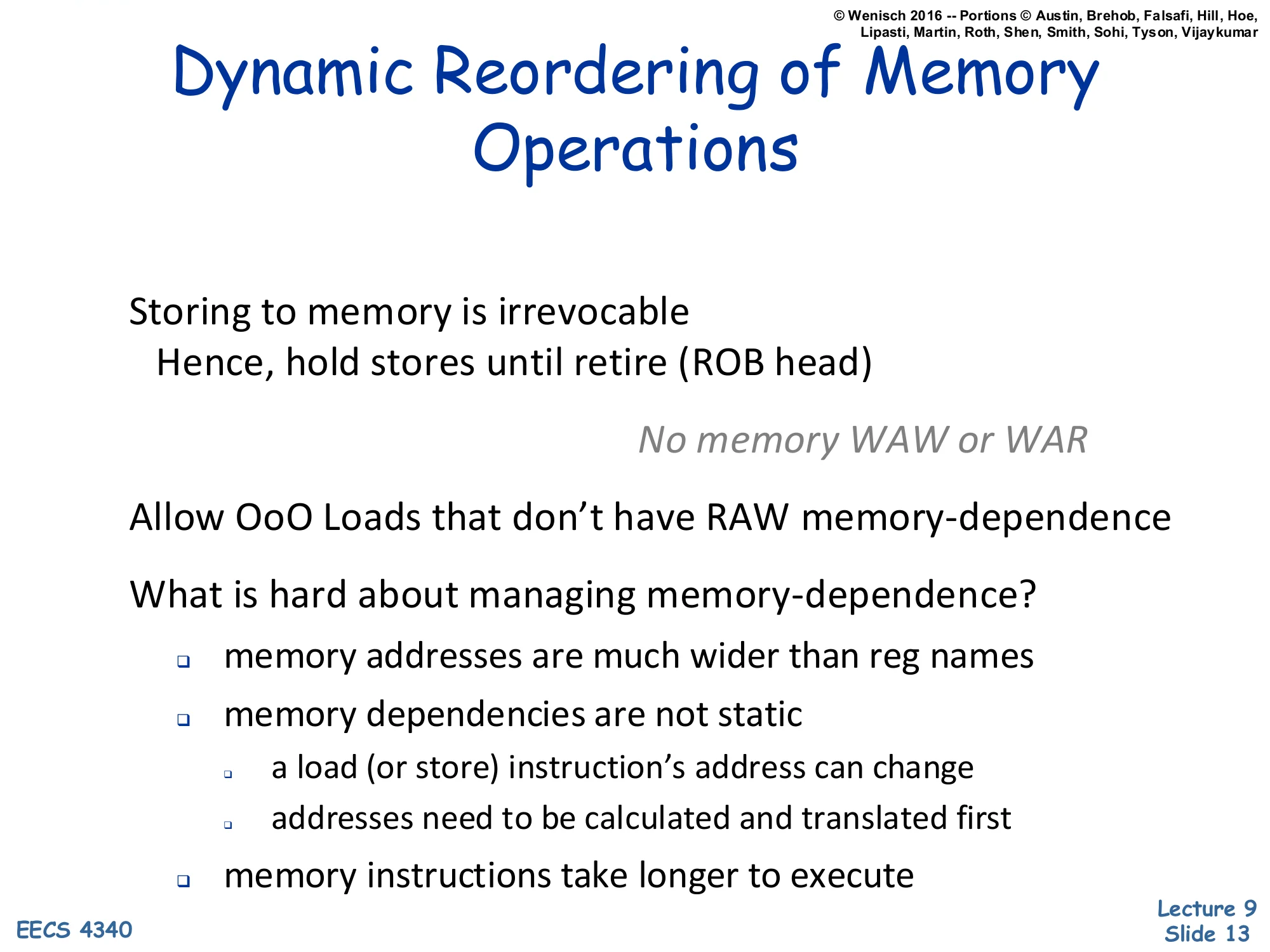
Dynamic Reordering of Memory Operations
- Storing to memory is irrevocable
- Hence, hold stores until retire (ROB head)
- No memory WAW or WAR
- Allow OoO Loads that don’t have RAW memory-dependence
- What is hard about managing memory-dependence?
- memory addresses are much wider than reg names
- memory dependencies are not static
- a load (or store) instruction’s address can change
- addresses need to be calculated and translated first
- memory instructions take longer to execute
Two design constants come from the irrevocability of memory writes. First, stores must wait until they retire (reach the ROB head) before updating the cache, because once a write hits memory, no rollback is possible — this is what holds stores in the store queue until commit. Second, because stores are never speculatively committed to memory, there are no memory-side WAW or WAR hazards: a younger store’s value cannot overwrite an older store’s value in the cache because both writes happen in retire order. That leaves only memory RAW as a real constraint: a load must observe the value of any older store to the same address. The slide also flags three reasons memory dependences are harder than register dependences: addresses are 32–64 bits (much wider than 5-bit register names), they are computed at execute time (not at decode), and memory operations take many cycles, so the dependence-detection window stays open longer.
Some trivial ways to handle Loads
Show slide text
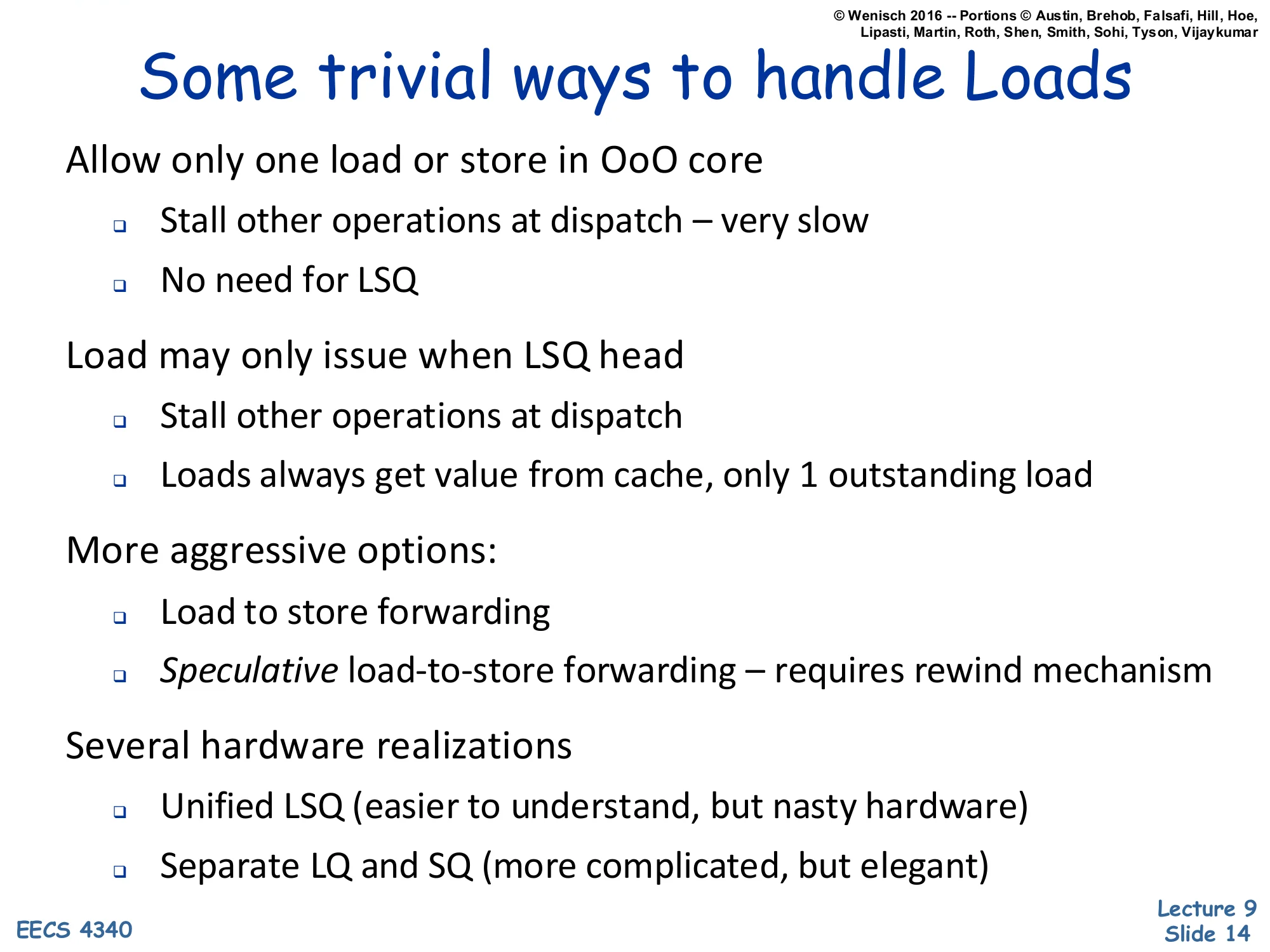
Some trivial ways to handle Loads
- Allow only one load or store in OoO core
- Stall other operations at dispatch — very slow
- No need for LSQ
- Load may only issue when LSQ head
- Stall other operations at dispatch
- Loads always get value from cache, only 1 outstanding load
- More aggressive options:
- Load to store forwarding
- Speculative load-to-store forwarding — requires rewind mechanism
- Several hardware realizations
- Unified LSQ (easier to understand, but nasty hardware)
- Separate LQ and SQ (more complicated, but elegant)
The slide enumerates the design space from “trivially correct” to “aggressively speculative.” Allowing only one in-flight memory operation is correct but throughput-killing — the OoO machine becomes serial on every load or store. A slightly better stand is to require loads to wait until they reach the LSQ head, which still serializes them. The first useful upgrade is load-to-store forwarding: when a load executes, its address is compared against older store-queue entries, and a hit lets the load take the store’s value directly without going to the cache. The most aggressive option is speculative load-to-store forwarding — let loads issue past stores whose addresses are still unknown, then detect and recover from any mispredicted bypass. The lecture will build to this last design through two hardware options: a unified LSQ (one structure with N×N comparators, conceptually simple but messy in silicon) and split LQ/SQ (separate queues, more complex protocol but cleaner physical design).
Recall: Load/Store Queue (LSQ)
Show slide text
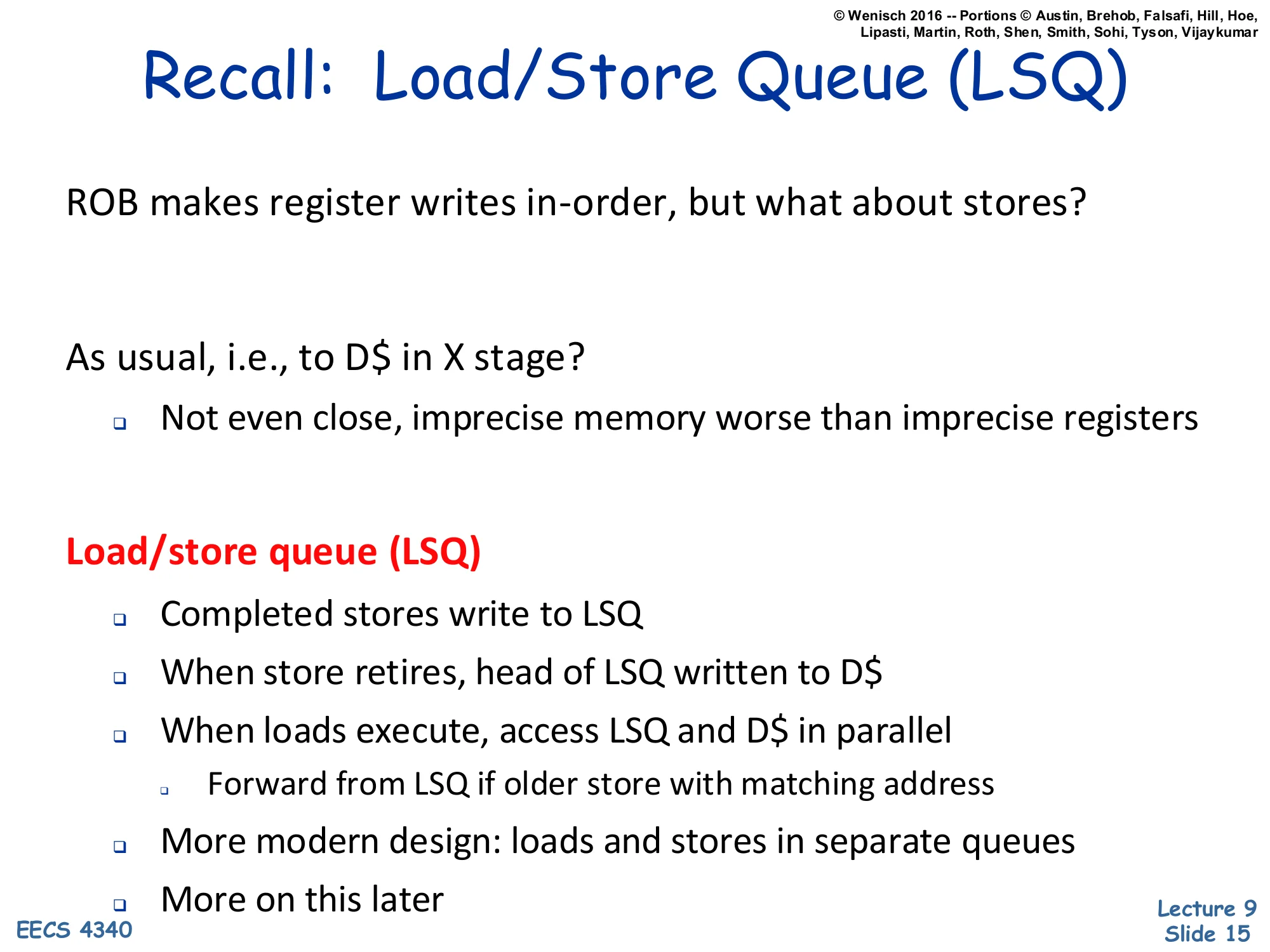
Recall: Load/Store Queue (LSQ)
ROB makes register writes in-order, but what about stores?
- As usual, i.e., to D$ in X stage?
- Not even close, imprecise memory worse than imprecise registers
- Load/store queue (LSQ)
- Completed stores write to LSQ
- When store retires, head of LSQ written to D$
- When loads execute, access LSQ and D$ in parallel
- Forward from LSQ if older store with matching address
- More modern design: loads and stores in separate queues
The slide reminds you why an LSQ is needed at all: if a store wrote the data cache during Execute, every speculative store on a mispredicted path would corrupt memory, and rolling memory back is essentially impossible — no architectural-map-table trick can undo an L1 write. The LSQ is therefore the memory-side analog of the ROB: completed stores write into the LSQ at execute time, but only at retire is the value pushed from the LSQ head into the D-cache. Loads, when they execute, query the LSQ and the cache in parallel — if an older store in the LSQ matches the load’s address, the load takes that store’s value (forwarding) instead of whatever the cache has, because the cache cannot yet have the in-flight store’s data. The closing line previews the split LQ/SQ design that the next slide and the worked example will build.
Recall: ROB + LSQ
Show slide text
Recall: ROB + LSQ
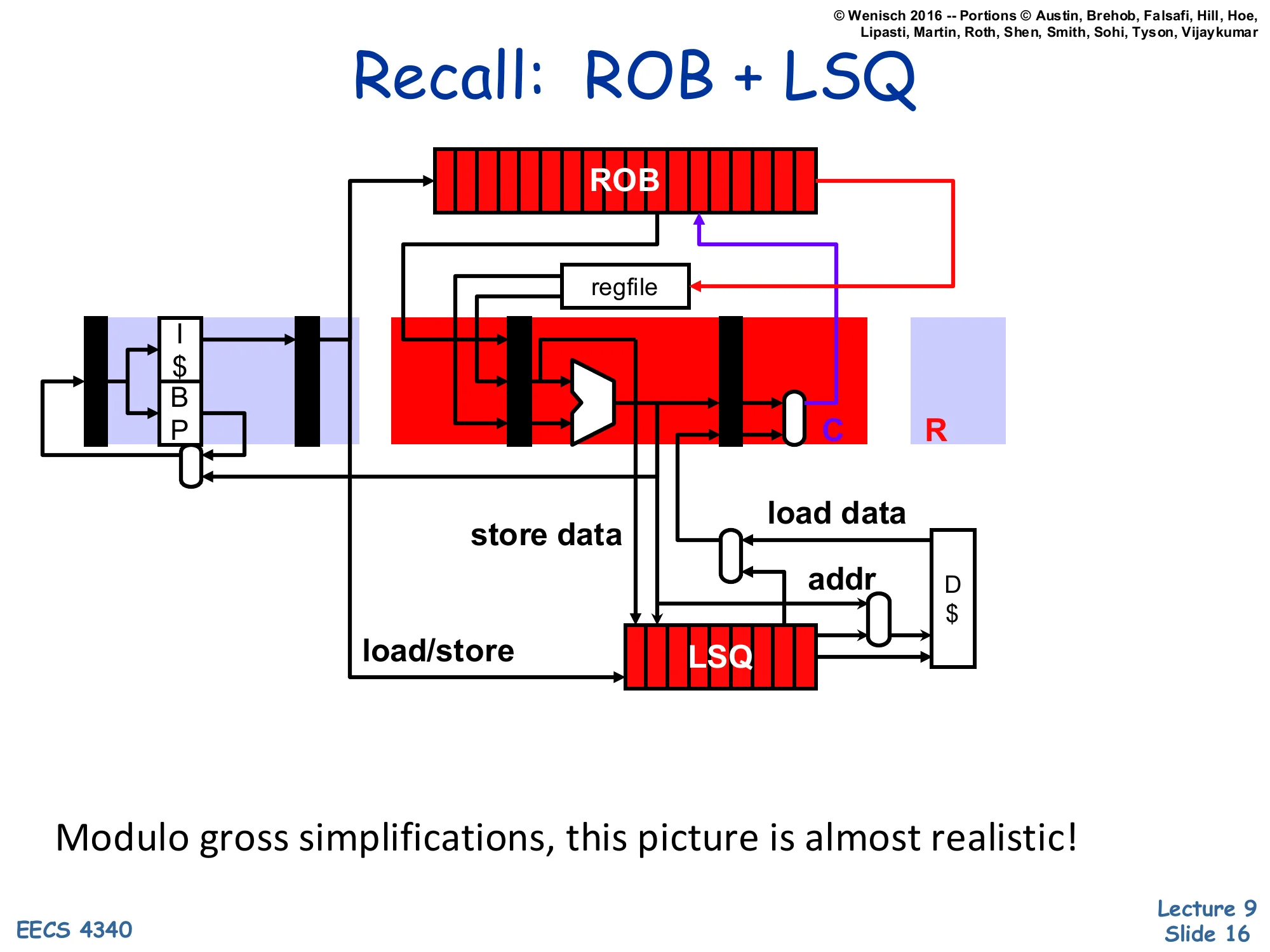
Datapath sketch: I-cache+BP feeds the ROB and regfile; the load/store unit produces store-data and addr that flow into the LSQ, which exchanges load-data with the D-cache and feeds the C/R (commit/retire) stage.
Modulo gross simplifications, this picture is almost realistic!
The block diagram shows where the LSQ sits in a complete OoO pipeline. Up top, the front end (I-cache, branch prediction) feeds the ROB and the register file, just like an arithmetic-only OoO design. The new piece is the load/store unit on the bottom path: address-generation produces an address, store-data routes through the LSQ, and load-data returns either from the cache or forwarded from the LSQ. The LSQ exchanges data with the D-cache only at retire (for stores) and at execute (for loads). The C/R label at the right shows that retire is the commit point that drains LSQ entries. The professor’s parenthetical “modulo gross simplifications” is honest: real designs split AGEN, TLB, port arbitration, and replay logic into many sub-pipelines, but the high-level data path is exactly as drawn.
HW #1: Unified Load/Store Queue
Show slide text
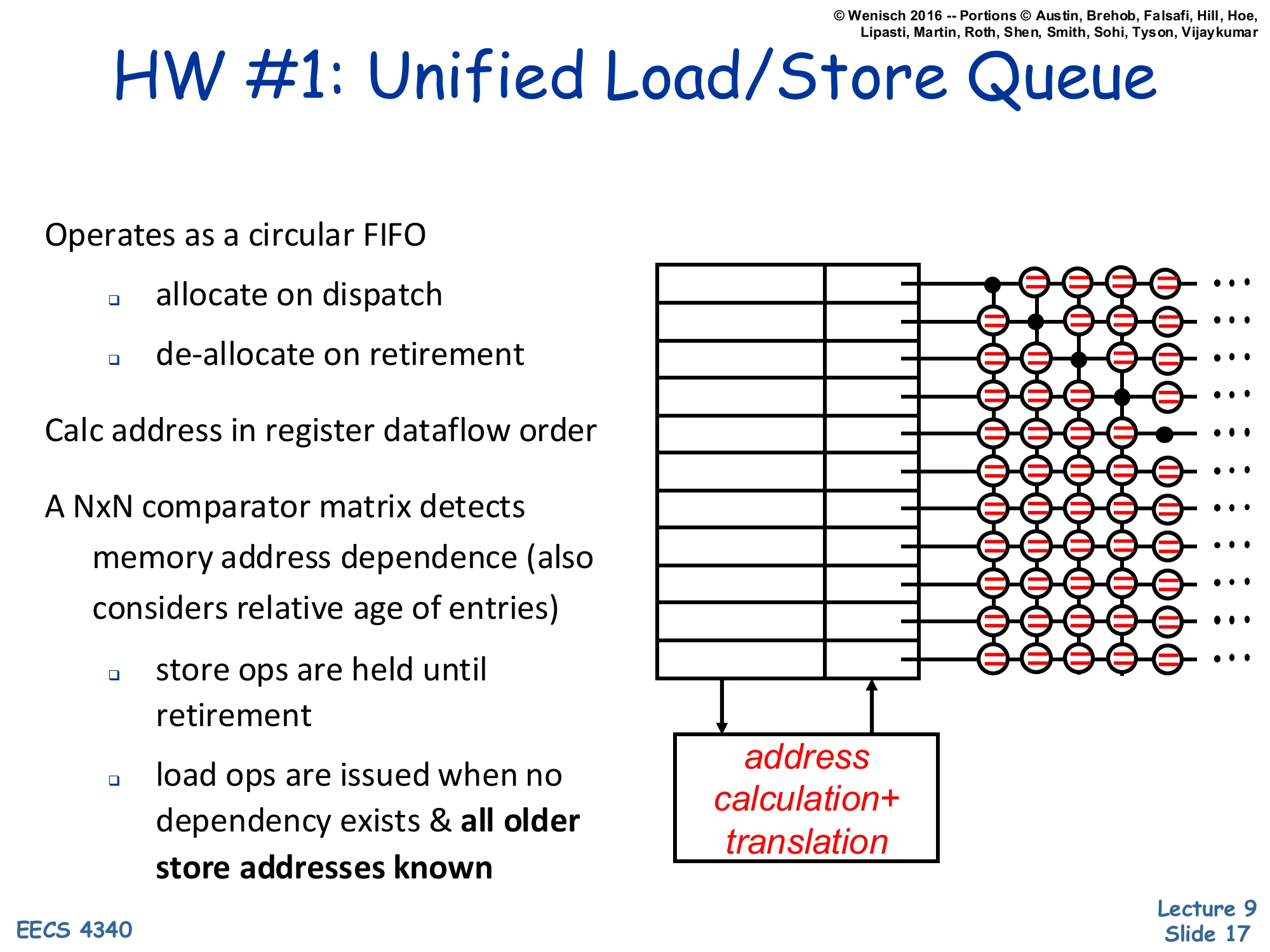
HW #1: Unified Load/Store Queue
- Operates as a circular FIFO
- allocate on dispatch
- de-allocate on retirement
- Calc address in register dataflow order
- A NxN comparator matrix detects memory address dependence (also considers relative age of entries)
- store ops are held until retirement
- load ops are issued when no dependency exists & all older store addresses known
Diagram: rows of = = = = comparators across the unified queue, with an address calculation + translation arrow feeding incoming addresses into the matrix.
The first hardware option puts loads and stores into the same circular FIFO and detects memory dependences with an N×N comparator matrix: every entry’s address is compared against every other entry’s address, while age bits decide which match wins. The matrix scales as O(N2) in area and power, which is its main drawback — even modest queues (say 64 entries) need 64×64 = 4096 comparators, all wide enough for full physical addresses. Once dispatch allocates a slot, address generation fills the address field in register-dataflow order (whenever the AGEN inputs are ready). Stores wait until retire to update the cache; loads wait until both their own address is computed and every older store’s address is known, then either forward from a matching older store or issue to the cache. This is a faithful but conservative implementation of memory disambiguation — no speculation over unknown stores.
HW#2: Split Queues
Show slide text
HW#2: Split Queues
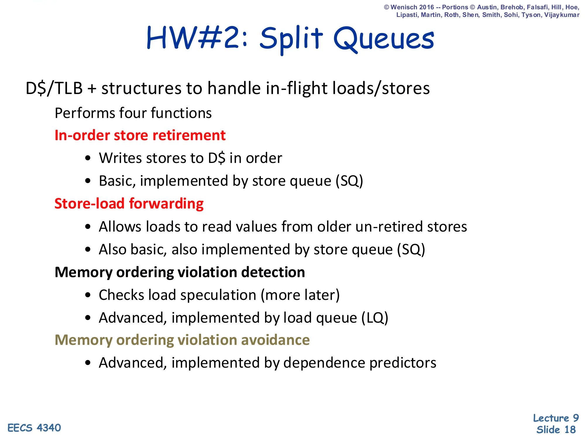
D$/TLB + structures to handle in-flight loads/stores
Performs four functions:
- In-order store retirement
- Writes stores to D$ in order
- Basic, implemented by store queue (SQ)
- Store-load forwarding
- Allows loads to read values from older un-retired stores
- Also basic, also implemented by store queue (SQ)
- Memory ordering violation detection
- Checks load speculation (more later)
- Advanced, implemented by load queue (LQ)
- Memory ordering violation avoidance
- Advanced, implemented by dependence predictors
The split-queue design factors the four memory-scheduling jobs cleanly across two structures and one predictor. The store queue (SQ) handles the two “basic” jobs — draining stores to the cache in program order at retire, and forwarding values to younger loads with matching addresses. The load queue (LQ) handles the “advanced” job — detecting memory ordering violations when a load was speculatively executed before an older same-address store. A separate dependence predictor handles the avoidance job — predicting which load/store pairs will conflict so the scheduler can keep them ordered without paying the penalty of a flush. The slide names the four jobs in increasing complexity; the rest of the lecture builds them up incrementally, starting with just the SQ (slides 19–23) and then layering on the LQ (slides 24–46) and dependence prediction (slides 47–48).
Simple Data Memory FU: D$/TLB + SQ

Show slide text
Simple Data Memory FU: D$/TLB + SQ
Inputs: address, data in, load position. Output: data out.
Just like any other FU:
- 2 register inputs (addr, data in)
- 1 register output (data out)
- 1 non-register input (load pos)?
Store queue (SQ):
- In-flight store address/value
- In program order (like ROB)
- Addresses associatively searchable
- Size heuristic: 15–20% of ROB
Layout: column of == comparators with address | value | age fields, head at top and tail at bottom, sitting above the D$/TLB.
But what does it do?
This slide treats the data-memory unit as just another functional unit with two register inputs (address and store-data) and one register output (load-data), plus one non-register input — the “load position” recorded at dispatch that tells later logic where this load sits in age order relative to the store queue. The SQ itself is a small in-program-order FIFO (15–20% of ROB size is the rule of thumb, since most instructions are not stores). Each entry holds an address, a value, and an age. The address column is associatively searchable — a CAM — so a load can broadcast its address and find any matching older store in one cycle. The slide poses the question “but what does it do?” because the SQ alone is just storage; the next slide describes the pipeline that drives it.
Data Memory FU "Pipeline"
Show slide text
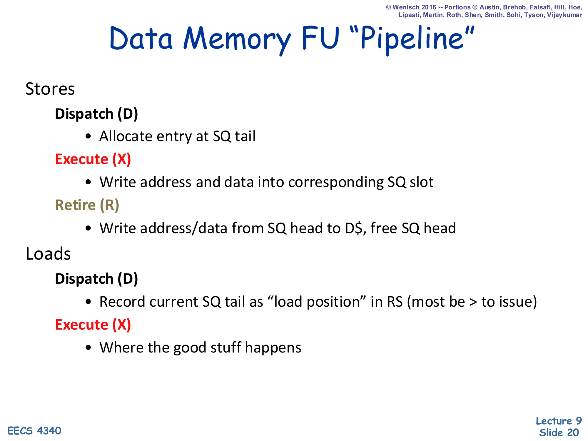
Data Memory FU “Pipeline”
Stores
- Dispatch (D)
- Allocate entry at SQ tail
- Execute (X)
- Write address and data into corresponding SQ slot
- Retire (R)
- Write address/data from SQ head to D$, free SQ head
Loads
- Dispatch (D)
- Record current SQ tail as “load position” in RS (most be > to issue)
- Execute (X)
- Where the good stuff happens
The data-memory pipeline has three milestones for stores and (initially) two for loads. A store reserves an SQ slot at dispatch (in program order), fills in its address and value when it executes, and finally drains from the SQ head to the D-cache when it retires (popping that head entry). A load’s dispatch step is special: it captures the current SQ tail index as its “load position,” which freezes the set of older stores at the moment of dispatch — any SQ entry with index < load position is older, anything ≥ load position is younger. The note “most be > to issue” means the load must wait until its own SQ-position becomes addressable (i.e., the relevant older stores are visible). At execute time, the load’s address probes both the D-cache and the SQ in parallel; the next slide describes that probe in detail.
"Out-of-Order" Load Execution
Show slide text
”Out-of-Order” Load Execution
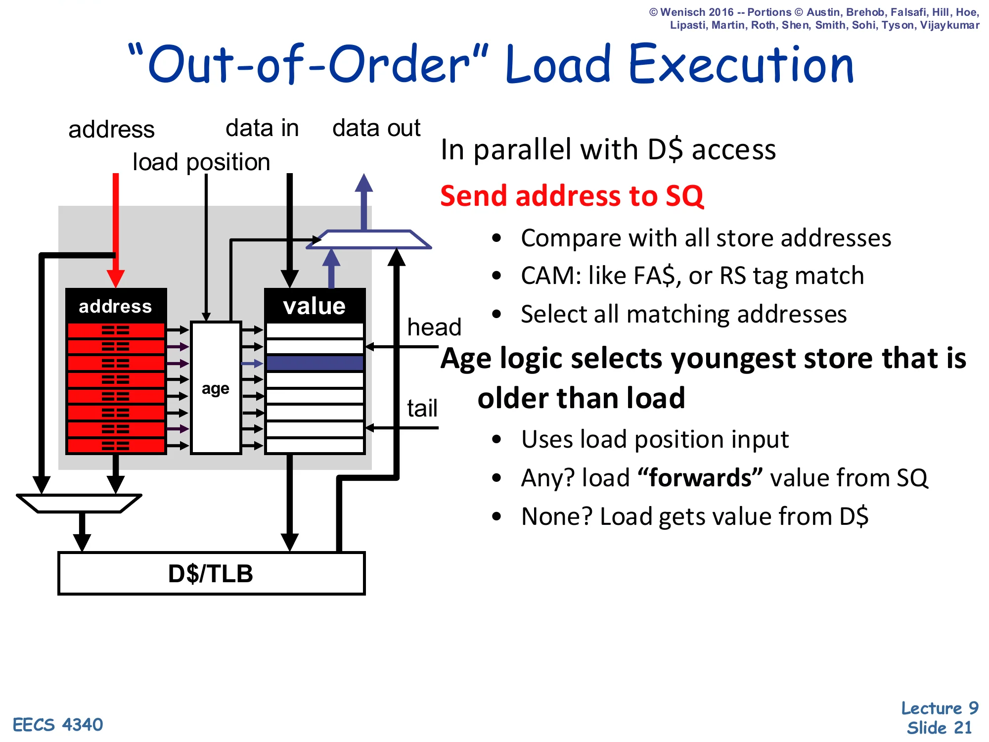
Inputs: address, data in, load position.
In parallel with D$ access:
- Send address to SQ
- Compare with all store addresses
- CAM: like FA$, or RS tag match
- Select all matching addresses
- Age logic selects youngest store that is older than load
- Uses load position input
- Any? load “forwards” value from SQ
- None? Load gets value from D$
This is the heart of store-to-load forwarding. While the D-cache (and TLB) lookup proceeds, the load’s address is also broadcast across the SQ CAM. Several older stores might match (e.g., if the program writes the same address twice before reading), so age logic compares each match’s SQ index against the load’s recorded load-position and selects the youngest store that is still older than the load — that’s the most recent producer the load should observe. If at least one match exists, the load takes the SQ value and discards the cache result; if none match, the cache value is correct. The slide notes that the CAM is structurally identical to a fully-associative cache or a reservation-station tag-match. Because all of this is conservative — the load only issues once all older store addresses are known — there’s no speculation yet, hence the scare quotes around “out-of-order”.
Conservative Load Scheduling
Show slide text
Conservative Load Scheduling
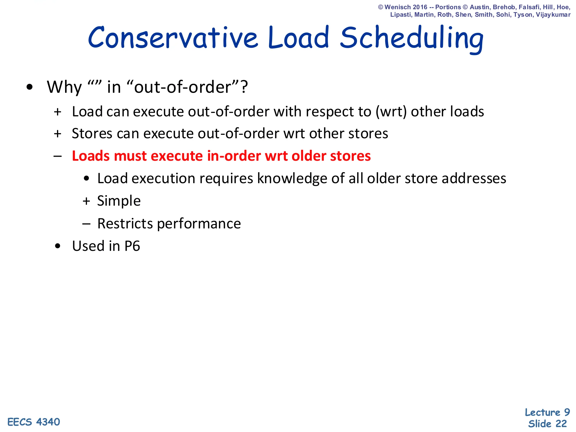
- Why "" in “out-of-order”?
-
- Load can execute out-of-order with respect to (wrt) other loads
-
- Stores can execute out-of-order wrt other stores
- – Loads must execute in-order wrt older stores
- Load execution requires knowledge of all older store addresses
-
- Simple
- – Restricts performance
-
- Used in P6
The slide explains why slide 21’s “out-of-order” was in scare quotes: this scheme allows reordering only in two of the three possible directions. Loads can pass other loads (because two loads can never alias each other in a way that violates ordering — they only read), and stores can compute their addresses out of order with respect to other stores (because stores still drain from the SQ in program order at retire). But loads cannot pass older stores — the load must stall until every older store’s address is known, otherwise disambiguation is impossible. The trade-off is simplicity (no speculation, no recovery, no detection logic) at the cost of performance (loads stall behind any slow address calculation in an older store). The P6 microarchitecture (Pentium Pro, Pentium II/III) used exactly this conservative scheme, which is part of why it never reached the clocks of contemporary R10K-style designs.
Opportunistic Memory Scheduling
Show slide text
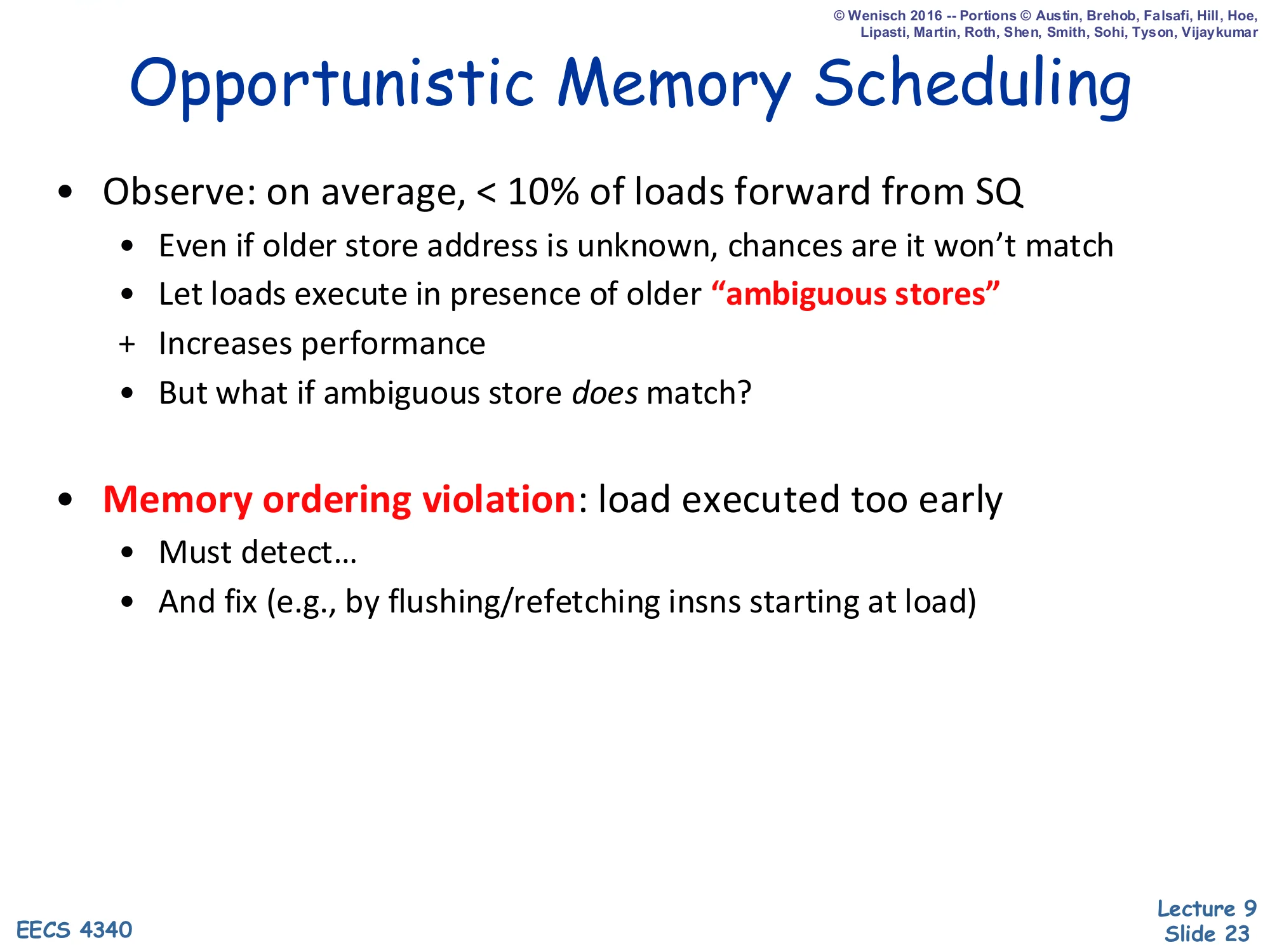
Opportunistic Memory Scheduling
- Observe: on average, < 10% of loads forward from SQ
- Even if older store address is unknown, chances are it won’t match
- Let loads execute in presence of older “ambiguous stores”
-
- Increases performance
- But what if ambiguous store does match?
- Memory ordering violation: load executed too early
- Must detect…
- And fix (e.g., by flushing/refetching insns starting at load)
Opportunistic scheduling is the speculative alternative to conservative scheduling. The empirical observation that drives it: in real programs, fewer than 10% of loads actually find a matching older store, so stalling every load until every older store address is known wastes cycles on the 90% of loads that would not have aliased anyway. The opportunistic policy is to let a load execute even when one or more older stores have unknown addresses (“ambiguous stores”). When a store later resolves its address, hardware checks the store queue against the load queue: any younger load that had already executed and would have matched this store is the victim of a memory ordering violation. The load (and everything younger) must be flushed and refetched. So opportunistic scheduling buys the common case (no flush) at the cost of a recovery mechanism for the uncommon case (misdisambiguation) — exactly the trade-off branch prediction makes for control flow.
D$/TLB + SQ + LQ
Show slide text
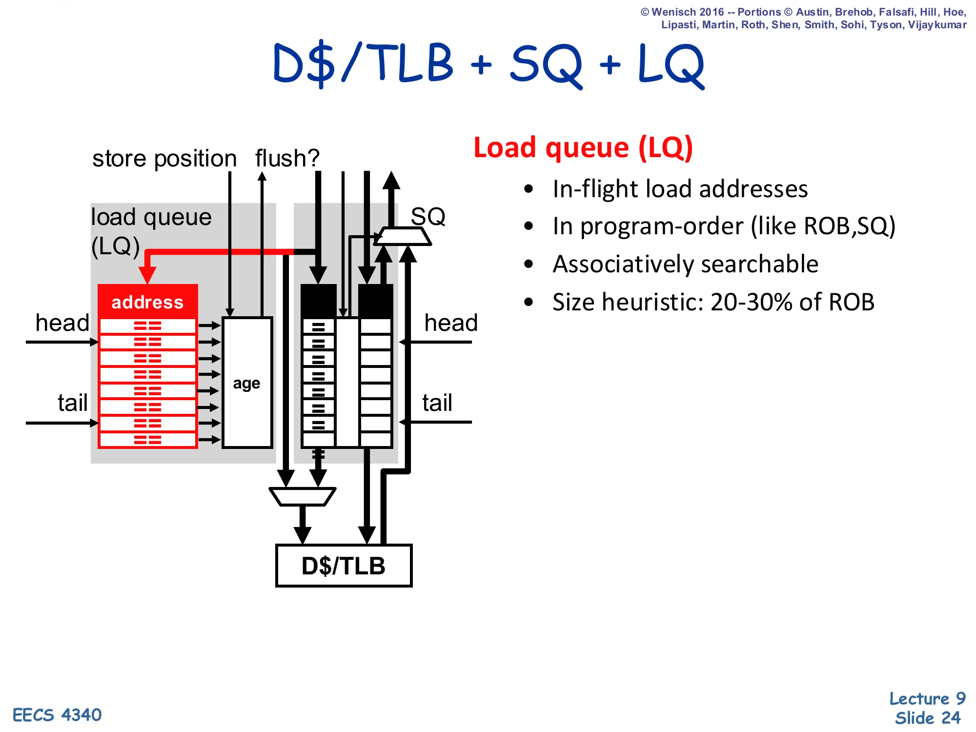
D$/TLB + SQ + LQ
New structure: load queue (LQ) sitting beside the SQ above the D$/TLB. Inputs include store position and flush?.
- Load queue (LQ)
- In-flight load addresses
- In program-order (like ROB, SQ)
- Associatively searchable
- Size heuristic: 20–30% of ROB
Layout: column of == comparators with an address field, age markers, head and tail pointers — symmetric mirror of the SQ.
Both SQ and LQ feed the D$/TLB on the right.
The opportunistic scheme requires a second queue — the load queue (LQ) — that records each in-flight load’s address so that a later store can search the LQ and detect if any younger load got the wrong value. Like the SQ, the LQ is in program order (mirroring the ROB) and is associatively searchable; its size (20–30% of ROB, larger than the SQ because loads outnumber stores in typical code) reflects load frequency. The new wires on the diagram are store position (the analog of “load position” — recorded at store dispatch so the store knows which LQ entries are younger than itself) and flush? (raised when the store’s address-broadcast finds a matching younger load that already executed, signaling a memory ordering violation). The LQ is the detection structure that opportunistic scheduling slides 22–23 promised.
Advanced Memory "Pipeline" (LQ Only)
Show slide text
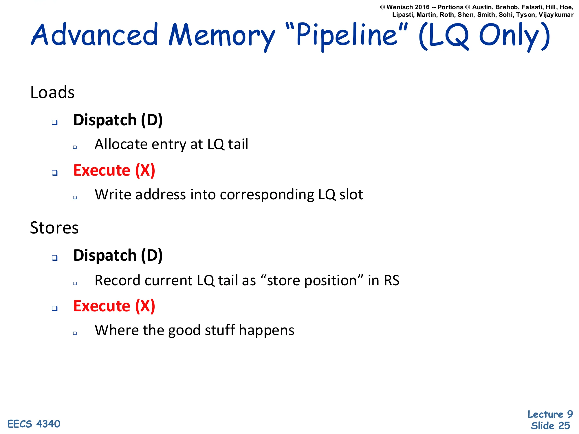
Advanced Memory “Pipeline” (LQ Only)
Loads
- Dispatch (D)
- Allocate entry at LQ tail
- Execute (X)
- Write address into corresponding LQ slot
Stores
- Dispatch (D)
- Record current LQ tail as “store position” in RS
- Execute (X)
- Where the good stuff happens
Adding the LQ adds a symmetric set of dispatch/execute steps for loads and stores. Loads now reserve an LQ slot at dispatch (so the slot exists for any later store to find) and write their address into that slot at execute time. Stores reserve their position via the LQ-tail snapshot at dispatch — recording “store position” as RS state — so when the store finally executes its address can be compared against exactly the LQ entries that are younger than it. Note that this slide shows only the LQ side of the pipeline; the SQ mechanics (slide 20) are unchanged and run in parallel. The combined pipeline lets a store-execute event trigger an LQ scan: any matching younger load that already executed is the victim of a memory ordering violation, and the next slide explains that detection logic.
Detecting Memory Ordering Violations
Show slide text
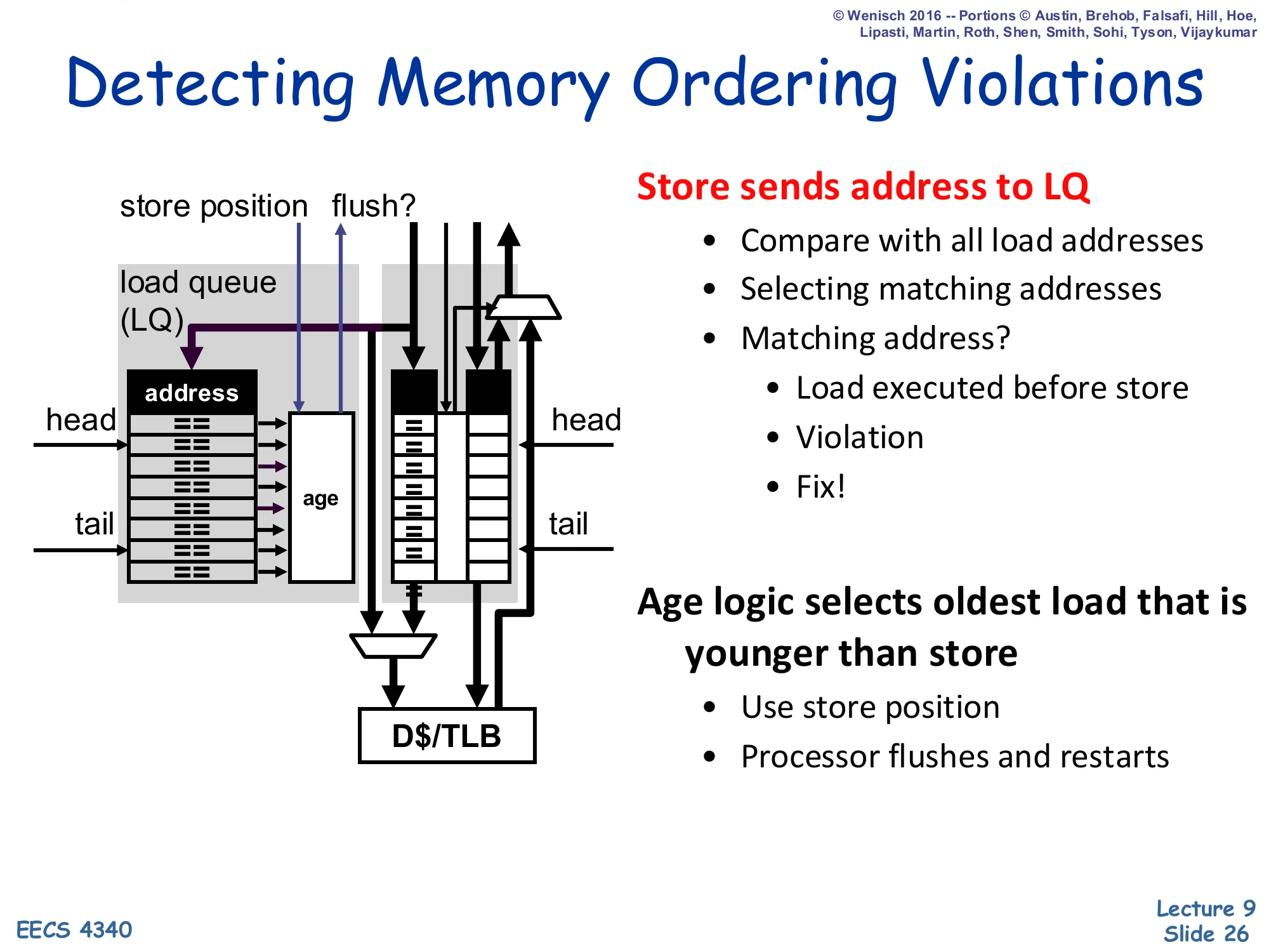
Detecting Memory Ordering Violations
Store sends address to LQ:
- Compare with all load addresses
- Selecting matching addresses
- Matching address?
- Load executed before store
- Violation
- Fix!
- Age logic selects oldest load that is younger than store
- Use store position
- Processor flushes and restarts
Diagram: store address fed into LQ CAM; matching loads identified via age logic; flush signal asserted to the front-end.
The detection algorithm is the dual of forwarding. When a store finally executes (its address resolved), it broadcasts its address into the LQ CAM. Any LQ entry whose address matches AND whose age is younger than the store’s (per the store’s recorded store-position) is a load that wrongfully executed before this store — it should have observed this store’s value but instead saw stale data. Age logic picks the oldest such victim load (the earliest-program-order violation), and the recovery action is a full pipeline flush and refetch starting at that load — the same recovery mechanism used for branch mispredictions. Because every younger instruction is also flushed, the design needs no fine-grained selective replay; this is the simplest and most common implementation of opportunistic memory disambiguation recovery, and it is the speculative fallback that justifies the LQ’s existence.
R10K Data Structures — Memory Example
Show slide text
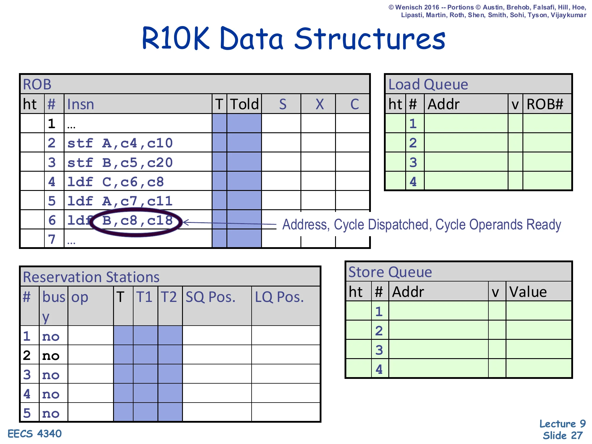
R10K Data Structures
ROB: 7 entries — 1 …, 2 stf A,c4,c10, 3 stf B,c5,c20, 4 ldf C,c6,c8, 5 ldf A,c7,c11, 6 ldf B,c8,c18, 7 … — columns T | Told | S | X | C.
Load Queue: 4 entries (Addr, v, ROB#) all blank.
Store Queue: 4 entries (Addr, v, Value) all blank.
Reservation Stations: 5 entries (bus | op | T | T1 | T2 | SQ Pos. | LQ Pos.), all no.
Legend: each insn shows Address, Cycle Dispatched, Cycle Operands Ready.
This kicks off the cycle-by-cycle worked example that occupies the next 19 slides. The trace mixes two stores and three loads. Two of the loads alias the stores — load 5 (ldf A) reads the address that store 2 just wrote, and load 6 (ldf B) reads the address that store 3 wrote — but in this example load 6 is going to issue before store 3’s address is resolved, triggering the memory ordering violation the previous slides described. The numbers next to each instruction encode (address, cycle dispatched, cycle operands ready), e.g. stf A,c4,c10 means store-A was dispatched at cycle 4 and its operands become ready at cycle 10. The ROB, SQ, and LQ all start empty and will fill up as dispatch progresses. The reservation-station columns now include SQ Pos. and LQ Pos. — the snapshot indices captured at dispatch that drive forwarding and violation detection.
Cycle 3

Show slide text
Cycle 3
ROB head/tail both at slot 1 (…). LQ empty (v=0 everywhere). SQ empty (v=0 everywhere). All RS entries no.
ROB rows show insns 1–7 in their initial state with no S/X/C cycles filled in yet. Load Queue and Store Queue both have ht 1 markers in slot 1 indicating head and tail co-located on the empty entry.
Cycle 3 is the first snapshot of the trace. Nothing has been dispatched into a memory queue yet — all four LQ slots and all four SQ slots show v=0 (empty/invalid). The ROB head and tail pointers both sit on the placeholder slot 1 (…), meaning we’re at the start of the relevant window. This is the baseline against which the next cycles will show queue allocations, address writes, and (eventually) the flush event. From cycle 4 onward, dispatch will start allocating SQ and LQ entries one per cycle as the seven instructions enter the back end.
Cycle 4 — first store dispatched
Show slide text
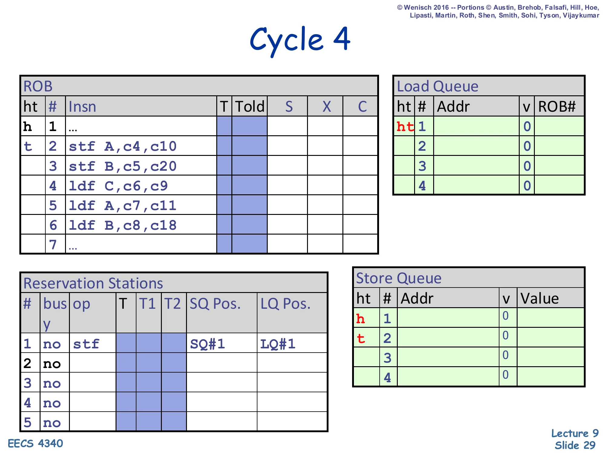
Cycle 4
ROB: head still at 1, tail advances to slot 2 (stf A,c4,c10).
Load Queue: head/tail markers h 1 / t 2 — first LQ entry reserved for the upcoming load.
Reservation Stations: RS#1 holds stf with SQ Pos. = SQ#1, LQ Pos. = LQ#1.
SQ: head/tail still at slot 1 — entry reserved but address/value not yet written.
Store 2 (stf A) dispatches in cycle 4. Three things happen simultaneously: the ROB tail advances to slot 2, the SQ tail advances reserving SQ#1 for this store, and the store’s reservation-station entry records SQ Pos. = SQ#1 (its own slot) and LQ Pos. = LQ#1 (the snapshot of the LQ tail at the moment of dispatch — meaning every LQ entry ≥ LQ#1 is younger than this store and thus a candidate for violation detection). The LQ tail is also advanced because the LSQ allocation scheme reserves slots conservatively; in this implementation the head pointer pins to LQ#1 even though no load has yet been dispatched. The store’s address (A) and value will not appear in the SQ until it executes at cycle 10 — for now the slot is just reserved.
Cycle 5 — second store dispatched
Show slide text
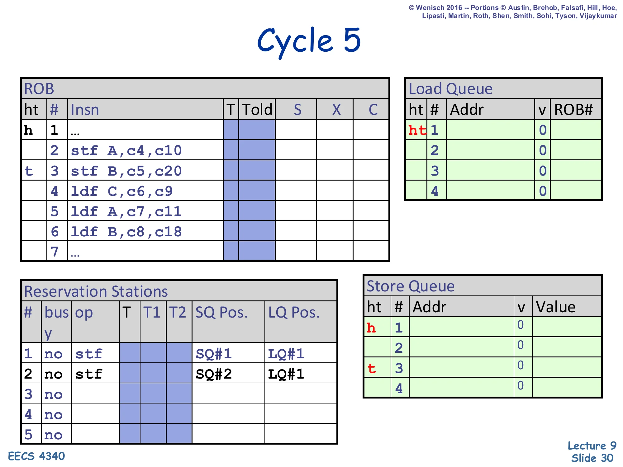
Cycle 5
ROB: head at 1, tail advances to slot 3 (stf B,c5,c20).
Reservation Stations:
- RS#1:
stf | SQ#1 | LQ#1 - RS#2:
stf | SQ#2 | LQ#1
SQ: head still at slot 1, tail advances to slot 3 — two SQ entries now reserved.
LQ: unchanged from cycle 4.
Store 3 (stf B) dispatches in cycle 5. The ROB tail advances to slot 3. The SQ tail moves to slot 3 (slot 2 was reserved for store 3). Each store records its own SQ Pos. and a snapshot of the current LQ tail as LQ Pos. Both stores in this trace see LQ Pos. = LQ#1 because no load has been dispatched yet — every LQ entry that ever appears will be younger than both stores. The SQ now has entries reserved for stores 2 and 3 in program order, but neither has an address or value yet because they have not executed.
Cycle 6 — first load dispatched
Show slide text
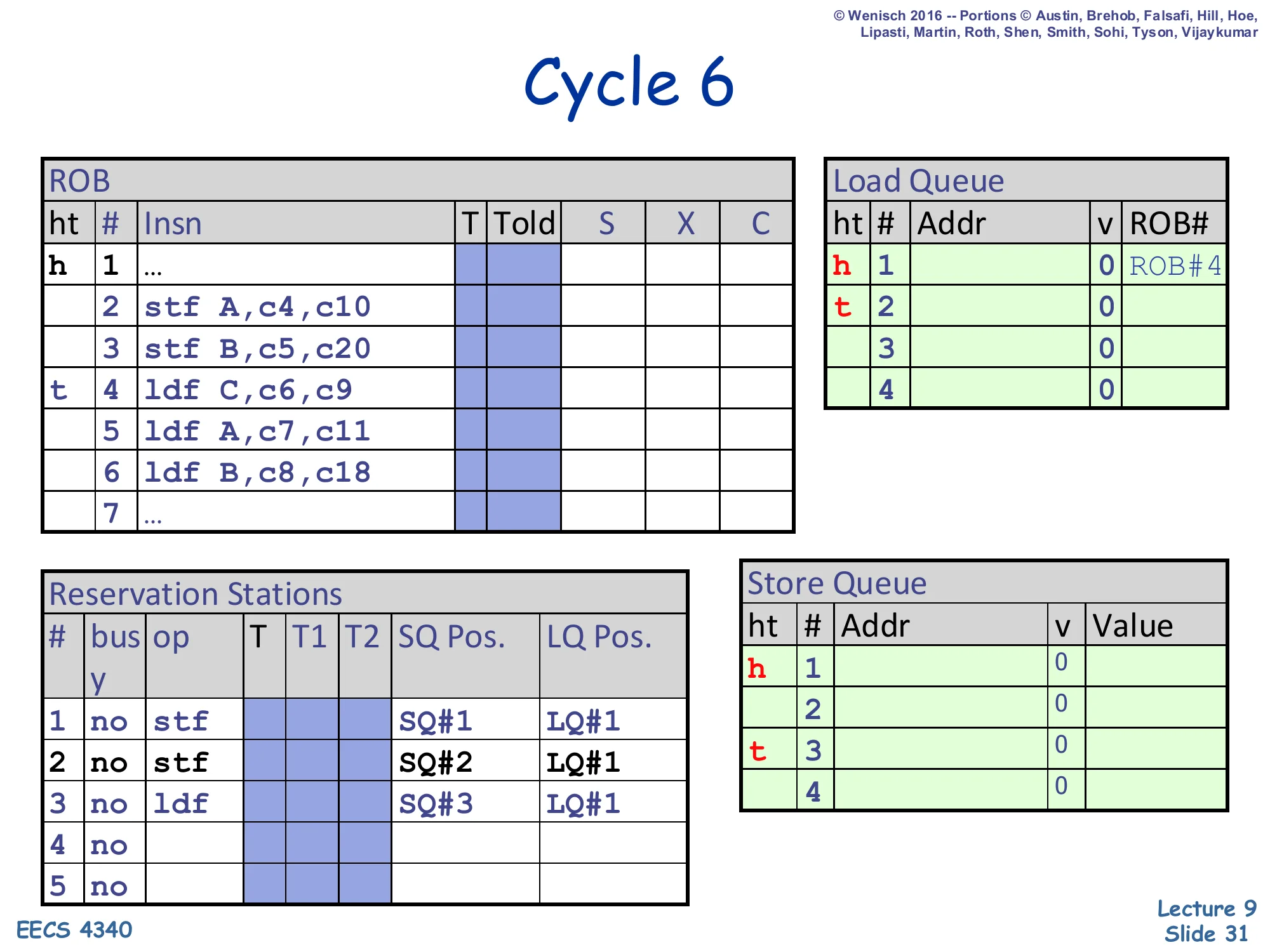
Cycle 6
ROB: head at 1, tail advances to slot 4 (ldf C,c6,c9).
Load Queue: head at slot 1, tail advances to slot 2 — first LQ entry reserved for ldf C.
Reservation Stations:
- RS#1:
stf | SQ#1 | LQ#1 - RS#2:
stf | SQ#2 | LQ#1 - RS#3:
ldf | SQ#3 | LQ#1
RS#3 records SQ Pos. = SQ#3 (current SQ tail) and LQ Pos. = LQ#1 (its own LQ slot).
Load 4 (ldf C) dispatches at cycle 6. Three things happen: the ROB tail advances to slot 4, an LQ slot (LQ#1) is reserved at the LQ tail for this load, and the load’s reservation-station entry captures SQ Pos. = SQ#3 (the current SQ tail, meaning every SQ entry with index < SQ#3 is older than this load) and LQ Pos. = LQ#1 (its own LQ slot). When this load executes, it will use SQ Pos. = SQ#3 to filter SQ matches to only older stores (SQ#1 and SQ#2). The LQ tail moves to slot 2 in preparation for the next load.
Cycle 7 — second load dispatched
Show slide text
Cycle 7
ROB: head at 1, tail advances to slot 5 (ldf A,c7,c11).
Load Queue: tail advances to slot 3 — second LQ entry reserved for ldf A.
Reservation Stations:
- RS#1:
stf | SQ#1 | LQ#1 - RS#2:
stf | SQ#2 | LQ#1 - RS#3:
ldf | SQ#3 | LQ#1 - RS#4:
ldf | SQ#3 | LQ#2
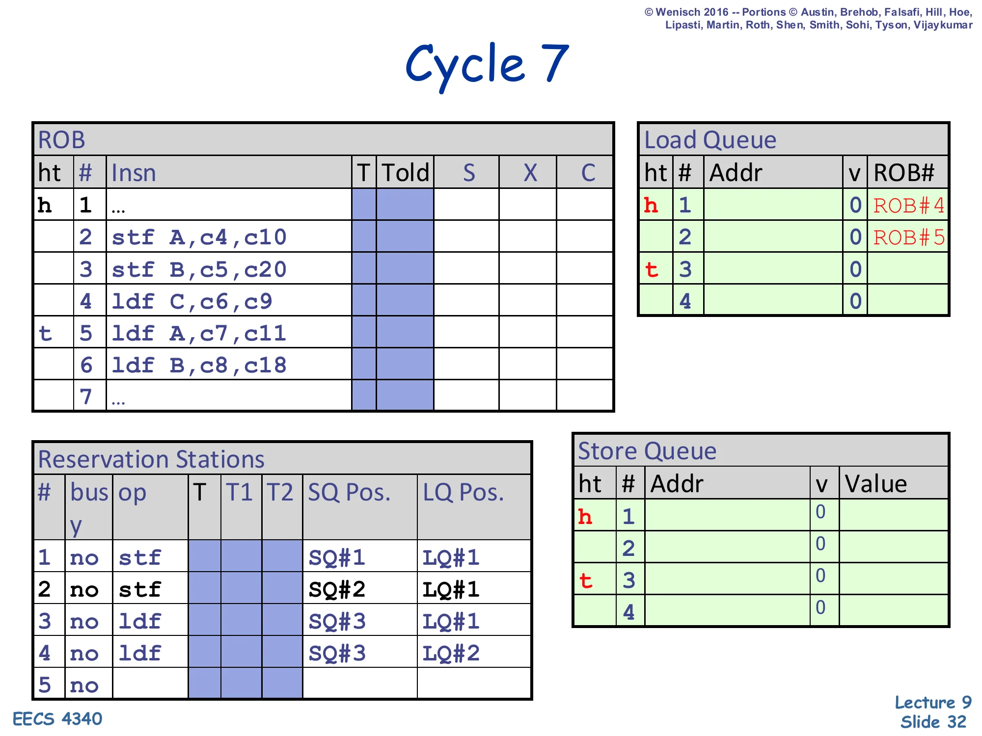
Load 5 (ldf A) dispatches at cycle 7 into LQ#2 with SQ Pos. = SQ#3 (same as load 4’s snapshot — still the SQ tail) and LQ Pos. = LQ#2. This load is the dangerous one: it reads address A, which is the address that store 2 will eventually write. Right now store 2’s address is not yet resolved (store 2 doesn’t execute until cycle 10), but the conservative scheme would force ldf A to wait. This trace is using the opportunistic scheme, so ldf A will be allowed to issue the moment its register operands are ready — at cycle 11 — even though store 2 has only just resolved (cycle 10) and store 3 has not. The ROB tail moves to slot 5.
Cycle 8 — third load dispatched

Show slide text
Cycle 8
ROB: head at 1, tail advances to slot 6 (ldf B,c8,c18).
Load Queue: tail advances to slot 4 — third LQ entry reserved for ldf B.
Reservation Stations:
- RS#1:
stf | SQ#1 | LQ#1 - RS#2:
stf | SQ#2 | LQ#1 - RS#3:
ldf | SQ#3 | LQ#1 - RS#4:
ldf | SQ#3 | LQ#2 - RS#5:
ldf | SQ#3 | LQ#3
Load 6 (ldf B) dispatches at cycle 8 into LQ#3 with SQ Pos. = SQ#3 and LQ Pos. = LQ#3. This load reads address B, which is what store 3 will write — but store 3’s address resolution is delayed all the way to cycle 20, while load 6’s operands become ready at cycle 18. So load 6 will execute long before store 3’s address is known, fetching the stale value of B from the cache. When store 3 finally executes at cycle 20 and broadcasts address B to the LQ, the disambiguation logic will spot the violation and trigger a flush. All five reservation stations are now occupied; the ROB tail is at slot 6.
Cycle 9 — first load issues
Show slide text
Cycle 9
ROB: head 1, tail 6. Slot 4 (ldf C) shows X = c9 — load C begins execution.
Reservation Stations:
- RS#3:
ldf | + + | SQ#3 | LQ#1(now ready, operands+)
LQ and SQ contents unchanged.
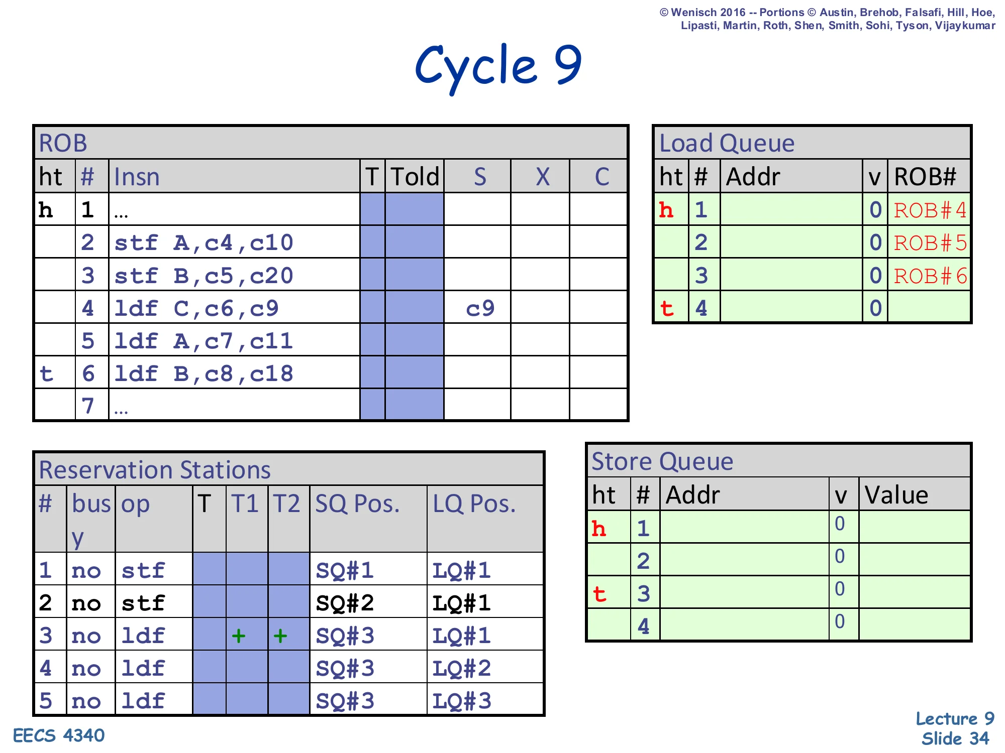
Load 4 (ldf C) — the only load to address C, which neither store touches — has both register operands ready at cycle 9 (the c6,c9 annotation: dispatched cycle 6, ready cycle 9), so its RS marks both T1 and T2 as ready (+) and it begins execution. The execute step writes the load’s address into LQ#1. Stores 2 and 3 have not yet executed, so the ambiguous-store check will rely on the opportunistic policy. Because load C’s address does not match any in-flight store’s address (and never will — no store touches C), even when stores eventually broadcast their addresses, no violation will fire for this load. This is the common-case 90% the lecture earlier called out: most loads don’t alias any in-flight store and so benefit from the speculative scheme without ever paying its recovery cost.
Cycle 10 — load C completes from cache
Show slide text
Cycle 10
ROB: slot 2 (stf A) shows X = c10 — store A begins execution. Slot 4 (ldf C) shows X = c9, c10 — load C continues.
Load Queue: head row now h 1 C | 1 | ROB#4 — load C’s address (C) and ROB# stored, valid bit set.
Reservation Stations: RS#1 (stf for store A) shows + + ready, others unchanged.
Note on slide: “No match on Addr, so get cache value [C]”.
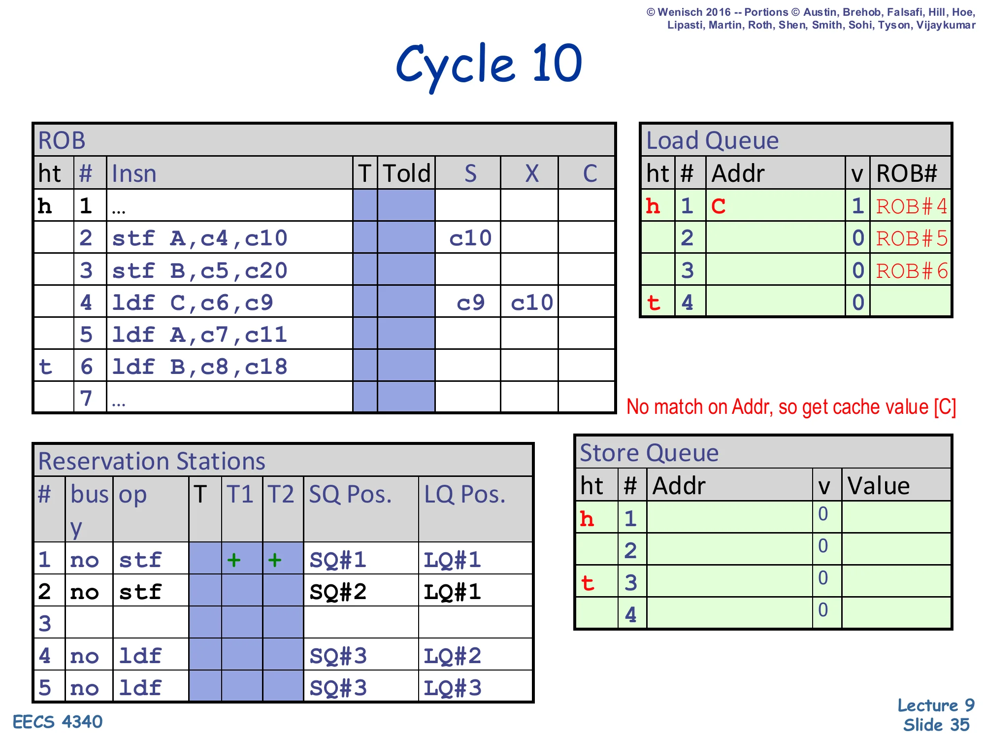
Two events at cycle 10. (1) Store 2 (stf A) becomes ready (its operands annotated c4,c10) and begins execution; its address A and value New A will be written into SQ#1 in the next cycle. (2) Load C completes its disambiguation check: it broadcasts address C into the SQ (which currently holds no addresses yet — both store entries are still empty), so there is no match and the load takes its value from the D-cache. The slide’s annotation “No match on Addr, so get cache value [C]” confirms the path. LQ#1 now records Addr = C, v = 1, ROB# = 4 so that later store-side checks know this LQ entry is valid and can be matched against future store addresses. The fact that load C completed correctly here illustrates why aggressive speculation is profitable: even with two ambiguous stores ahead of it, no violation occurred.
Cycle 11 — store A writes SQ, load A issues
Show slide text
Cycle 11
ROB:
- Slot 2 (
stf A): X showsc10, c11 - Slot 4 (
ldf C): X showsc9, c10, c11 - Slot 5 (
ldf A): X =c11— load A begins execution
Reservation Stations:
- RS#2:
stf | SQ#2 | LQ#1(still pending) - RS#4:
ldf | + + | SQ#3 | LQ#2(now ready)
Store Queue: head row h 1 A | 1 | New A — store A’s address A and value New A are now in SQ#1.
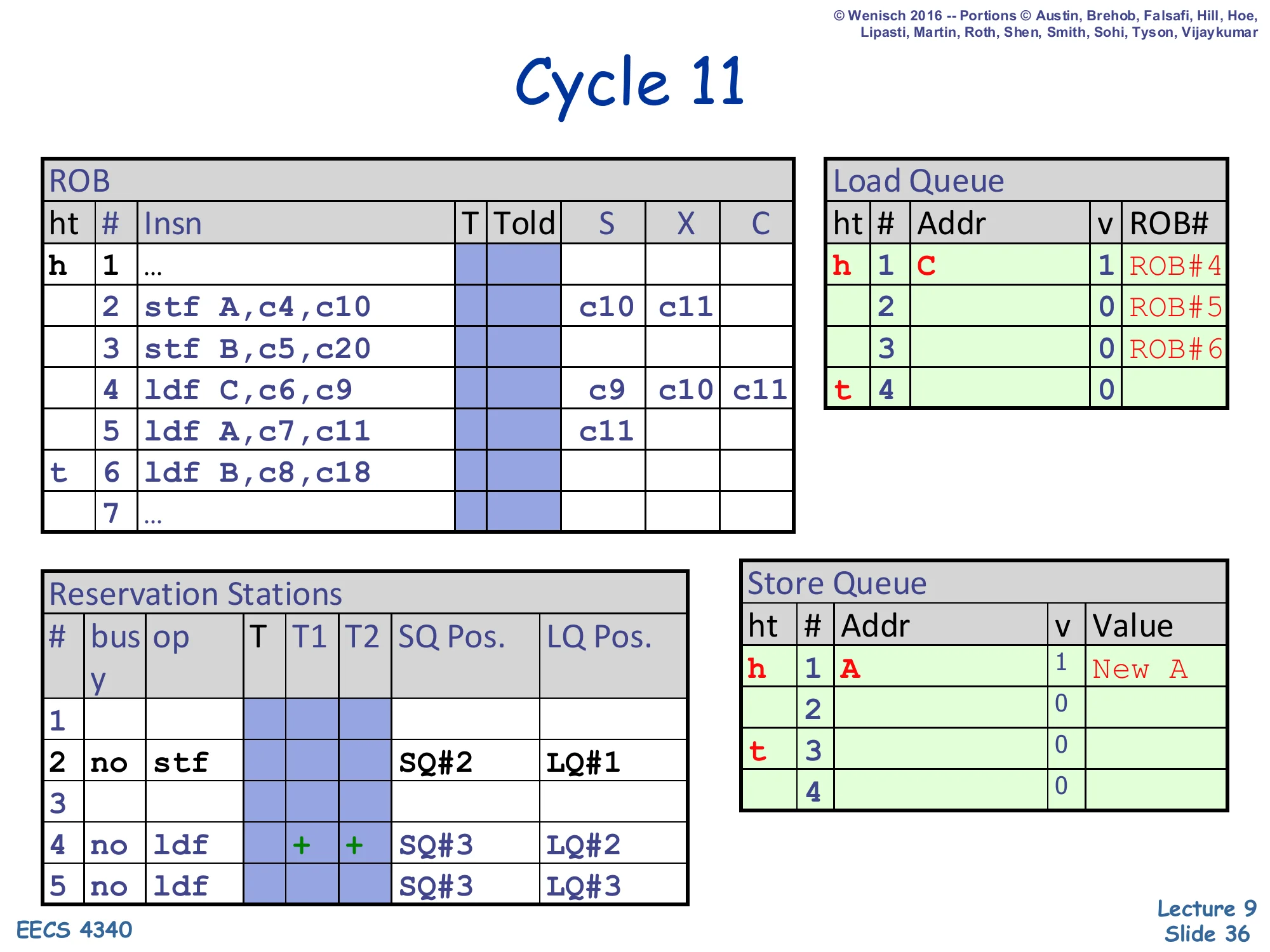
Two events at cycle 11. (1) Store A finishes its execute write — SQ#1 now holds Addr = A, valid, Value = New A. (2) Load 5 (ldf A) becomes ready (operands c7,c11) and begins to execute. The next slide will show what happens when this load checks the SQ for older same-address stores: it should hit on SQ#1 (older than this load via the load’s recorded SQ Pos. = SQ#3) and forward New A instead of going to the cache. Note that store 3 (stf B) is still un-executed — it has reserved SQ#2 but its address and value are unknown. This is exactly the “ambiguous store” situation: load 6 (ldf B) will see SQ#2 as an unknown-address older store but, under the opportunistic scheme, speculate past it anyway.
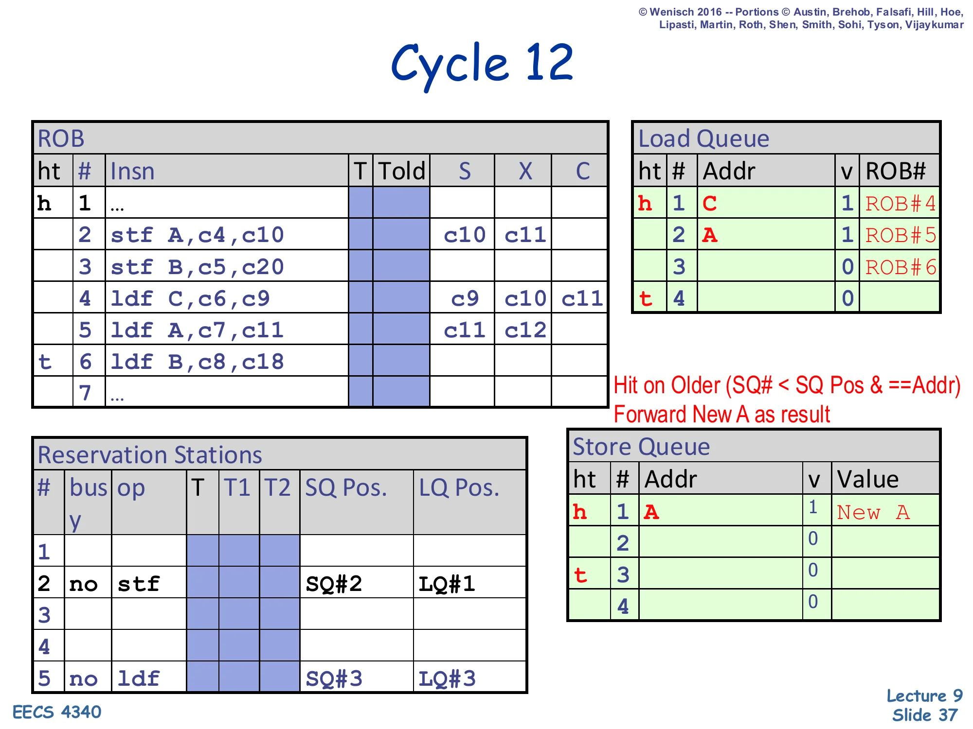
Cycle 12 — load A forwards from SQ
Show slide text
Cycle 12
ROB: slot 5 (ldf A): X shows c11, c12 — load A finishes.
Load Queue:
- LQ#1:
C | 1 | ROB#4 - LQ#2:
A | 1 | ROB#5(newly written)
Note on slide: “Hit on Older (SQ# < SQ Pos & ==Addr) — Forward New A as result.”
Reservation Stations: RS#5 (load B) still pending. RS#4 has retired its slot.
Load 5 (ldf A) executes in cycle 12 and runs the SQ CAM check. It finds SQ#1 with Addr = A and SQ# = 1 < load's SQ Pos = 3, meaning SQ#1 is an older store with the matching address — exactly the forwarding case from slide 21. Load A takes New A from the SQ rather than from the cache. The annotation Hit on Older (SQ# < SQ Pos & == Addr) makes the age and address conditions explicit. Load A’s address A is also written into LQ#2 with its valid bit set and ROB# = 5 — this is critical for the next check, because when store 3 eventually broadcasts B, store 3’s check will scan all LQ entries and confirm none of them match B. Forwarding here demonstrates the SQ’s basic store-load-forwarding job correctly handling a true memory RAW dependence.
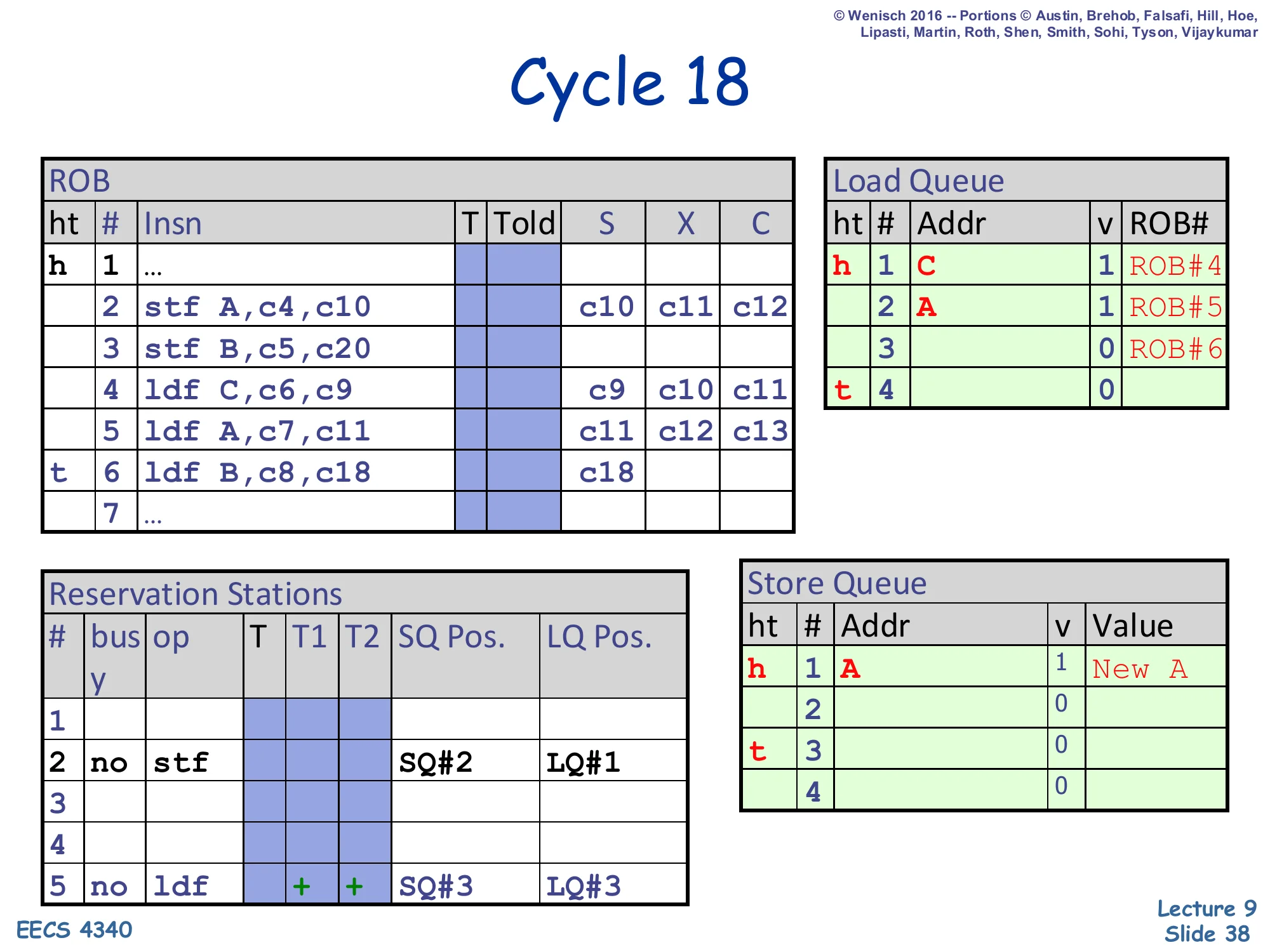
Cycle 18 — load B issues from cache
Show slide text
Cycle 18
ROB:
- Slot 2 (
stf A): X =c10, c11, c12 - Slot 5 (
ldf A): X =c11, c12, c13 - Slot 6 (
ldf B): X =c18— load B begins execution
Reservation Stations: RS#5 ldf | + + | SQ#3 | LQ#3 (ready).
Several cycles have passed (the trace skips from 12 to 18 because nothing visible happens in the middle). Load 6 (ldf B) finally has its operands ready at cycle 18 (its annotation was c8,c18) and begins to execute. At this moment, store 3 (stf B) is still unexecuted — its SQ entry SQ#2 has no address or value. Under the opportunistic scheme, load B issues anyway: it will scan the SQ, see only SQ#1 (with address A, no match) and SQ#2 (no address yet, ambiguous), and choose to speculate past the ambiguous SQ#2, taking the cache value of B. Note that this cache value is the stale B — store 3 is going to overwrite B with New B in two cycles — so this load is about to commit a memory ordering violation that will only be detected when store 3 finally executes.
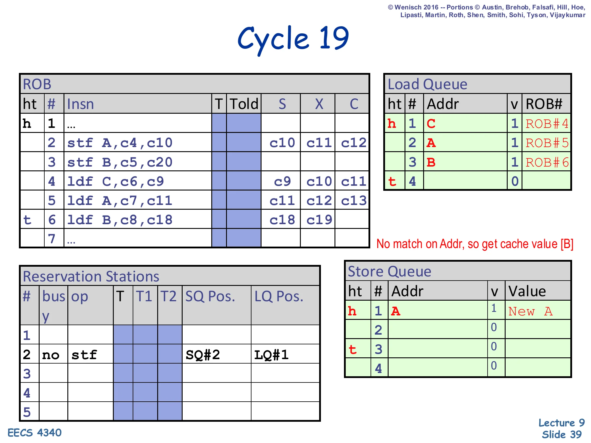
Cycle 19 — load B completes (incorrectly)
Show slide text
Cycle 19
ROB: slot 6 (ldf B): X = c18, c19.
Load Queue:
- LQ#1:
C | 1 | ROB#4 - LQ#2:
A | 1 | ROB#5 - LQ#3:
B | 1 | ROB#6(newly written)
Note on slide: “No match on Addr, so get cache value [B]”.
Load 6 (ldf B) finishes its execute step. Its address B is written into LQ#3, valid bit set, ROB# = 6. The SQ scan reports no match — SQ#1’s address is A (no match), SQ#2’s address is unknown — so under the opportunistic policy the load takes the cache value of B. The slide’s annotation “No match on Addr, so get cache value [B]” makes this concrete. This is the critical mistake: the cache holds the old value of B, but store 3 is about to put New B into SQ#2 in just one more cycle. The hardware does not yet know it has misdisambiguated — that knowledge only arrives after store 3 executes and triggers the LQ check that the next two cycles will show.
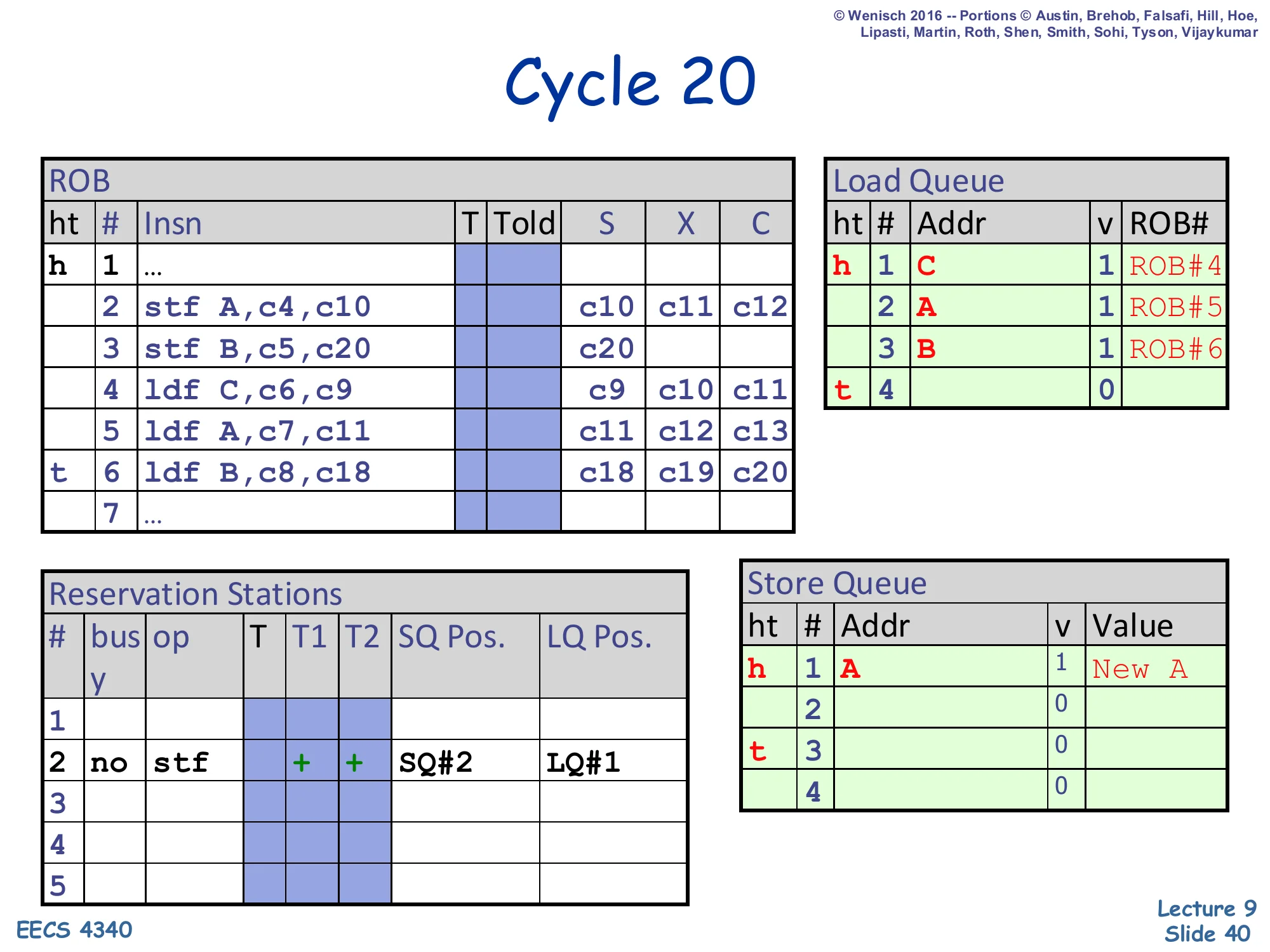
Cycle 20 — store B executes
Show slide text
Cycle 20
ROB:
- Slot 3 (
stf B): X =c20— store B begins execution. - Slot 6 (
ldf B): X =c18, c19, c20
Reservation Stations: RS#2 stf | + + | SQ#2 | LQ#1 (now ready).
LQ unchanged. SQ unchanged (entry SQ#2 still has no address).
Store 3 (stf B) finally has its operands ready (c5,c20) and begins to execute. Its reservation-station entry shows SQ Pos. = SQ#2 (its own SQ slot) and LQ Pos. = LQ#1 (LQ tail at the moment store 3 dispatched, way back at cycle 5 — so any LQ entry with index ≥ LQ#1 is younger than this store, which is all of LQ#1, LQ#2, LQ#3). On the next cycle, store 3 will write B and New B into SQ#2 and simultaneously broadcast B to the LQ. That LQ scan is what will detect the violation against load 6 (LQ#3). For now, both stores 2 and 3 have begun execute and load 6 has already executed with the stale cache value — the violation is locked in but not yet caught.
Cycle 21 — violation detected
Show slide text
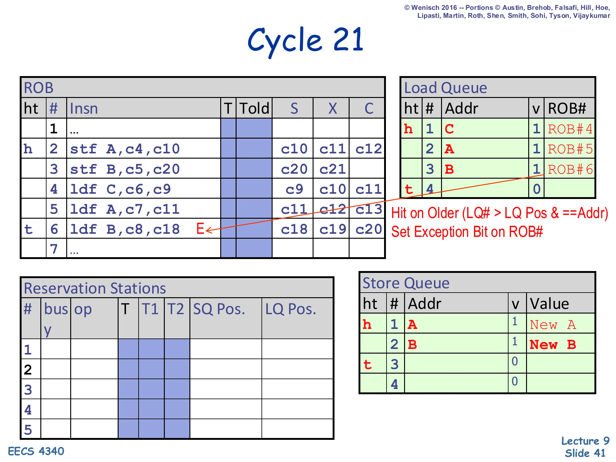
Cycle 21
ROB:
- Slot 3 (
stf B): X =c20, c21 - Slot 6 (
ldf B): now marked withEexception bit
Notes on slide:
- “Hit on Older (LQ# > LQ Pos & ==Addr)”
- “Set Exception Bit on ROB#”
Store Queue: SQ#1 (A, value New A, valid), SQ#2 (B, value New B, valid).
This is the violation-detection moment. Store 3 has just written its address B and value New B into SQ#2 and broadcast B across the LQ CAM. The LQ scan finds LQ#3 (B, valid, ROB#6) with LQ# = 3 > store's LQ Pos = 1, meaning LQ#3 is younger than the store. The condition LQ# > LQ Pos & == Addr triggers — load 6 already executed but should have observed this store. Hardware sets the exception bit E on ROB#6 (the load’s ROB entry). The actual flush is deferred until that ROB entry reaches the head and retires (cycle 26 in this trace), so younger instructions can keep retiring earlier results until the violation point is reached. This is the memory ordering violation that the opportunistic-scheduling slides described, now visible end-to-end in the trace.
Cycle 22 — store A retires
Show slide text
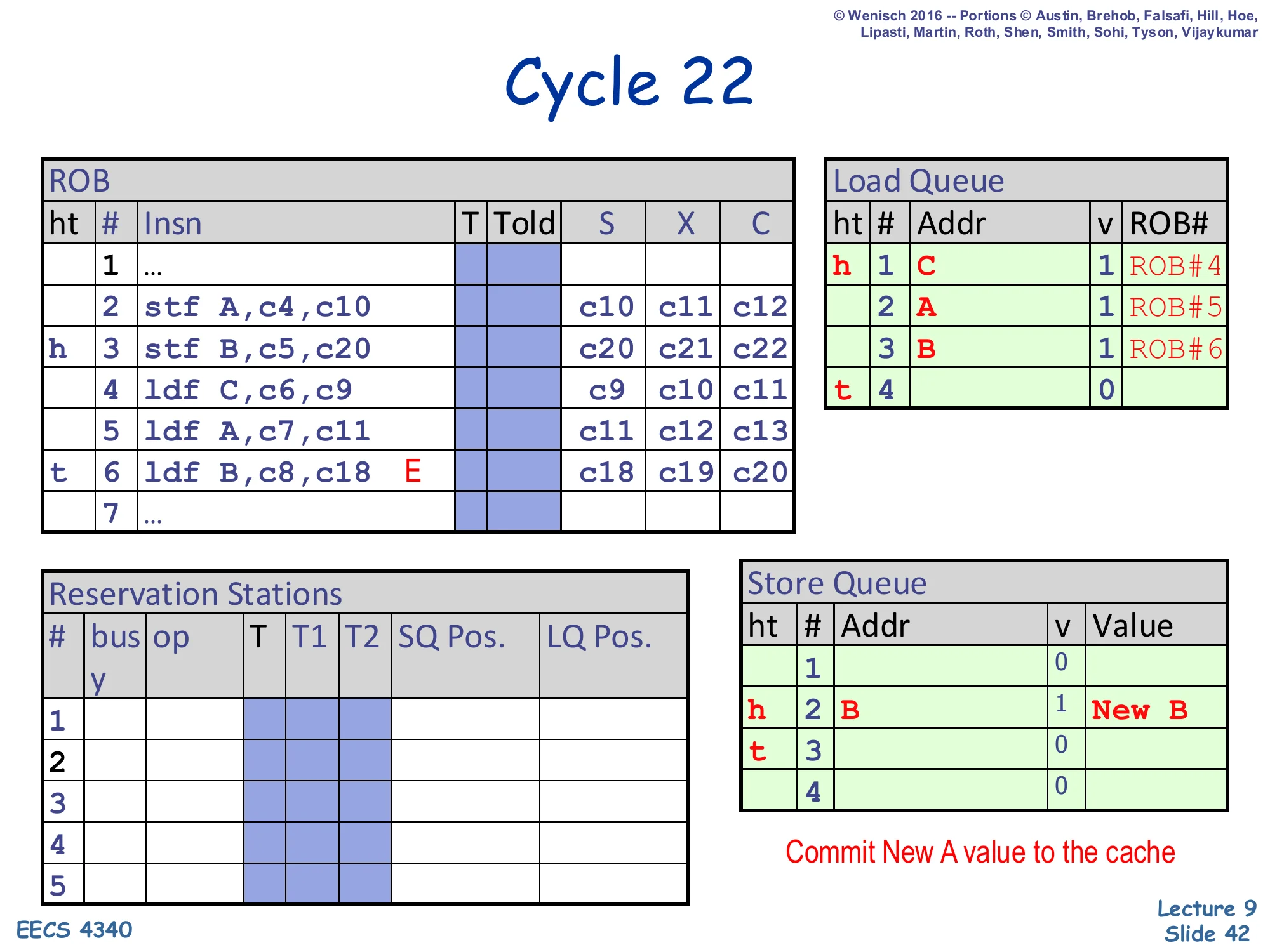
Cycle 22
ROB:
- Slot 2 (
stf A): X =c10, c11, c12(head; will be retired this cycle) - Slot 3 (
stf B): X =c20, c21, c22 - Slot 6 (
ldf B): still markedE
Store Queue:
- SQ#1 retired (slot 1 now invalid)
- SQ#2 (
B,New B, valid) becomes head
Note on slide: “Commit New A value to the cache”.
Store 2 reaches the ROB head and retires. The retirement action drains SQ#1 — the store’s address A and value New A are written to the D-cache. SQ#1 is now invalid and SQ#2 (the still-valid store-B entry) becomes the SQ head. From a memory-consistency viewpoint, this is the moment store A’s effect becomes globally visible. Note that even though store 3 has finished executing, it cannot retire yet because store 2 sits ahead of it in the ROB; stores must commit in program order. The exception bit on slot 6 still hasn’t fired because slot 6 has not reached the head yet — the flush is delayed until retire.
Cycle 23 — store B retires
Show slide text
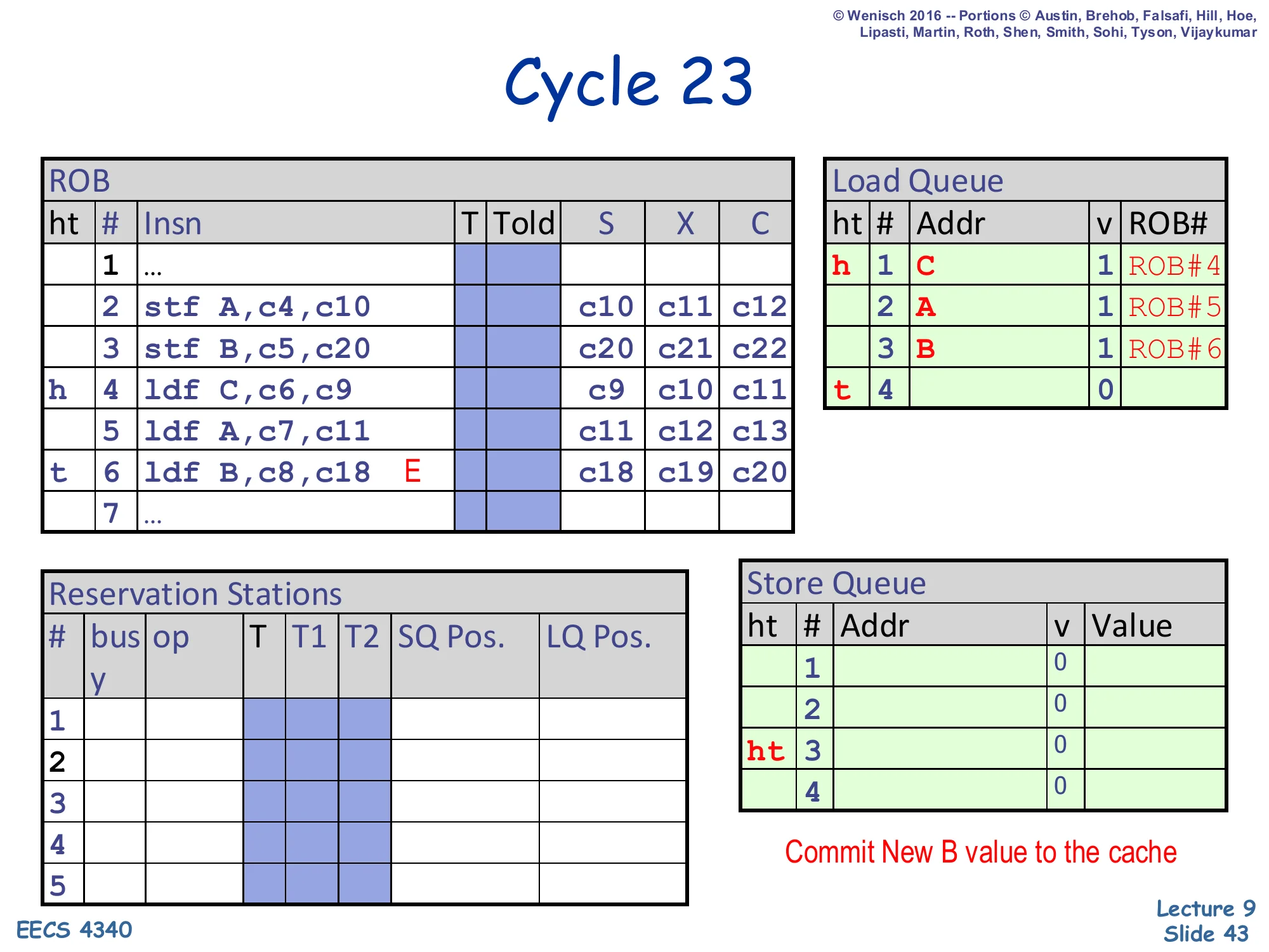
Cycle 23
ROB:
- Slot 3 (
stf B): head; retiring. - Slot 4 (
ldf C): next. - Slot 6: still
E.
Store Queue:
- SQ#1: invalid
- SQ#2: invalid (just retired)
- SQ#3: now head/tail (also invalid)
Note on slide: “Commit New B value to the cache”.
Store 3 reaches the ROB head and retires. SQ#2 drains — the store’s address B and value New B are written to the D-cache. The cache now holds New A and New B — both stores are globally visible. Critically, the SQ is now empty (only SQ#3 remains as a placeholder slot, also invalid). The next ROB head is slot 4 (load C), which will retire normally. Slots 5 and 6 (load A and the violating load B) follow. The flush at slot 6 is still queued via its exception bit; it will fire when slot 6 reaches the head.
Cycle 24 — load C retires
Show slide text
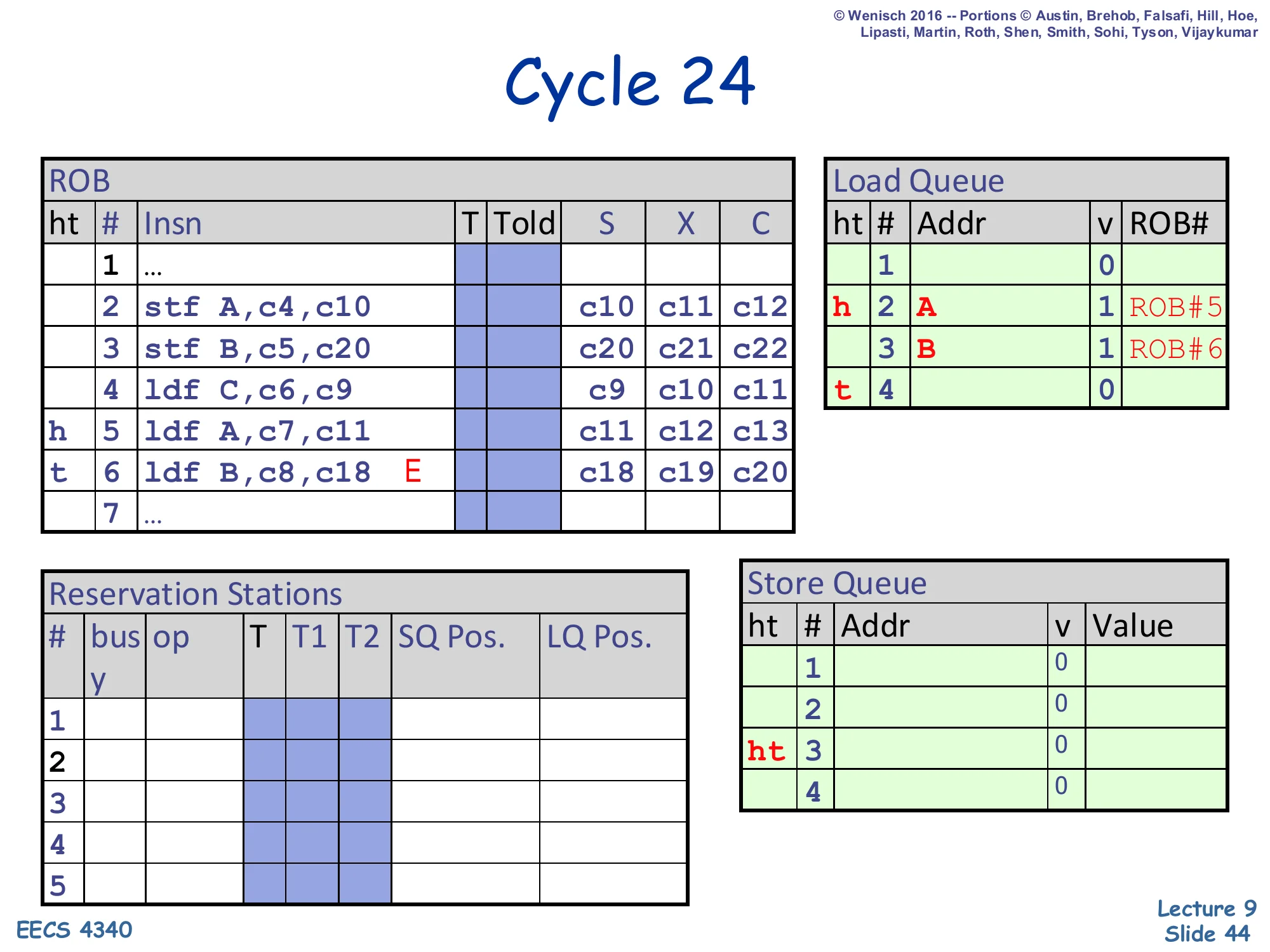
Cycle 24
ROB:
- Slot 4 (
ldf C): just retired. - Slot 5 (
ldf A): now head. - Slot 6: still
E.
Load Queue:
- LQ#1 invalid (just retired)
- LQ#2 (
A, valid, ROB#5) is new head
Load C reaches the ROB head and retires normally — its result was correct (cache value of C), so no flush. LQ#1 drains; LQ#2 (load A) becomes the new LQ head. Note the elegant invariant: every retiring load drains exactly one LQ entry, just as every retiring store drains exactly one SQ entry. The next ROB head is load A (slot 5), which forwarded from SQ#1 in cycle 12 and got the correct New A, so it too will retire normally in the next cycle.
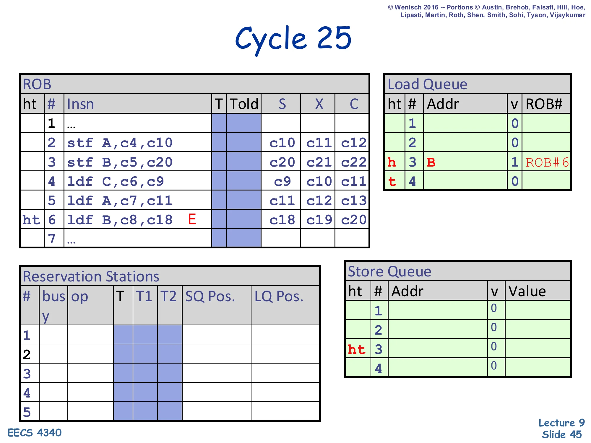
Cycle 25 — load A retires
Show slide text
Cycle 25
ROB:
- Slot 5 (
ldf A): just retired. - Slot 6 (
ldf B,E): now head and tail (ht).
Load Queue:
- LQ#2 invalid
- LQ#3 (
B, valid, ROB#6) is new head
Reservation Stations: empty.
Load A retires. LQ#2 drains and LQ#3 (the violating load B) becomes the LQ head and is also the ROB head/tail (ht 6). The pipeline has been steadily draining; the only thing left is the doomed load B. On the next cycle, when slot 6 retires, the exception bit will fire and the flush will execute. Notice that the ROB and LSQ have done their jobs perfectly: out-of-order execution overlapped store and load execution efficiently, the SQ correctly forwarded New A to load A, the LQ recorded all loads’ addresses, and the cycle-21 disambiguation check stamped the violation without disturbing the sequential retire order.
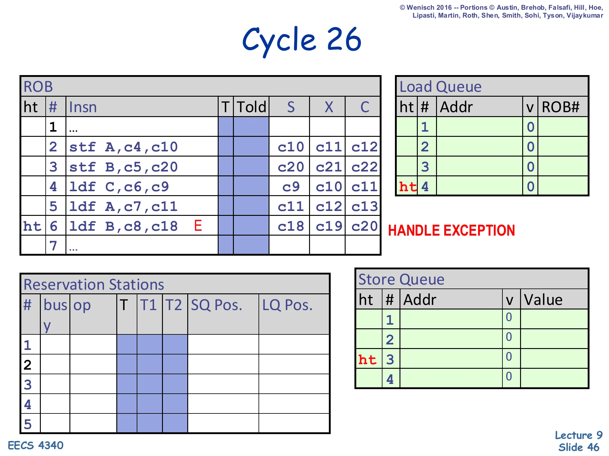
Cycle 26 — exception handled
Show slide text
Cycle 26
ROB: all entries cleared; head/tail markers move to slot 4.
Slot 6: still flagged E — “HANDLE EXCEPTION”.
Load Queue: all entries invalid; head/tail at LQ#4 (empty).
Store Queue: empty.
Slot 6 reaches the ROB head and the exception bit fires: the processor flushes everything from load B onward and refetches starting at the offending load. After the flush, every queue is empty: LQ has no in-flight loads, SQ has no in-flight stores, RS is idle. The load will be re-executed under the now-known correct memory state — store B’s New B is already in the cache (committed at cycle 23), so the second-time execution of load B will hit the cache and read New B correctly. The total cost of this memory ordering violation was the cycles between load B’s wrongful execute (cycle 18) and the flush (cycle 26) — eight cycles of wasted speculative work — plus the refetch latency. That is why slide 47 will note that opportunistic scheduling “introduces a few flushes, but each is much costlier than a delay,” motivating intelligent dependence prediction.
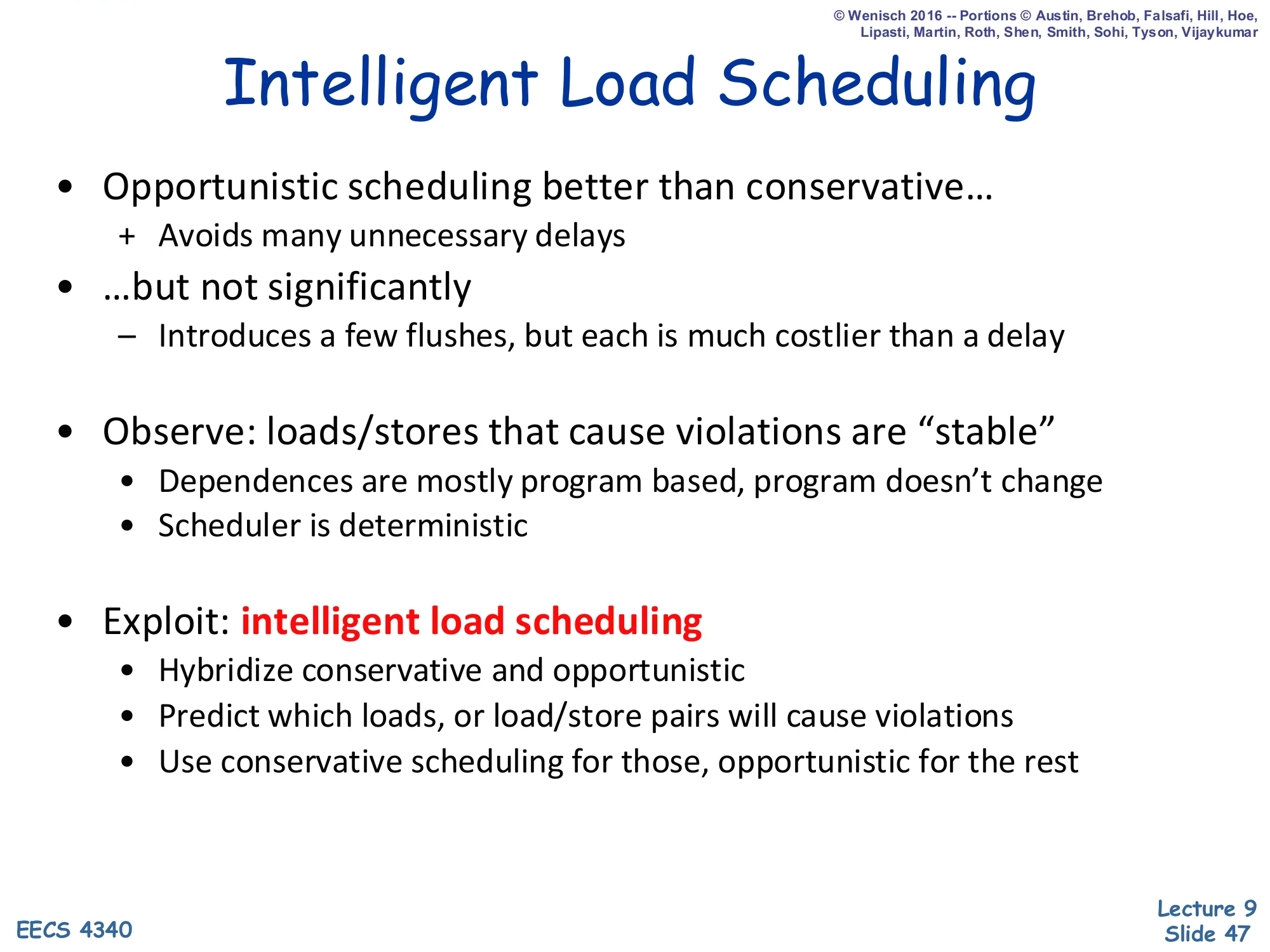
Intelligent Load Scheduling
Show slide text
Intelligent Load Scheduling
- Opportunistic scheduling better than conservative…
-
- Avoids many unnecessary delays
-
- …but not significantly
- – Introduces a few flushes, but each is much costlier than a delay
- Observe: loads/stores that cause violations are “stable”
- Dependences are mostly program based, program doesn’t change
- Scheduler is deterministic
- Exploit: intelligent load scheduling
- Hybridize conservative and opportunistic
- Predict which loads, or load/store pairs will cause violations
- Use conservative scheduling for those, opportunistic for the rest
The opportunistic scheme just demonstrated wins on average — most loads don’t alias, so few stall and few flush — but each flush costs many cycles, which can swamp the savings. The key empirical insight is that the loads that do cause violations are stable across executions: the same static load PC tends to alias the same static store PC every time the program runs through that path. So the violations are predictable. The intelligent-load-scheduling design is a hybrid: keep a small predictor that learns which loads (or which load/store pairs) have caused violations recently, and use the conservative policy for those — wait for older stores’ addresses — while letting all other loads use the opportunistic disambiguation policy. This turns rare-but-expensive flushes into one predicted stall per offending load, restoring most of the opportunistic gain. The next slide walks through two concrete predictor schemes.
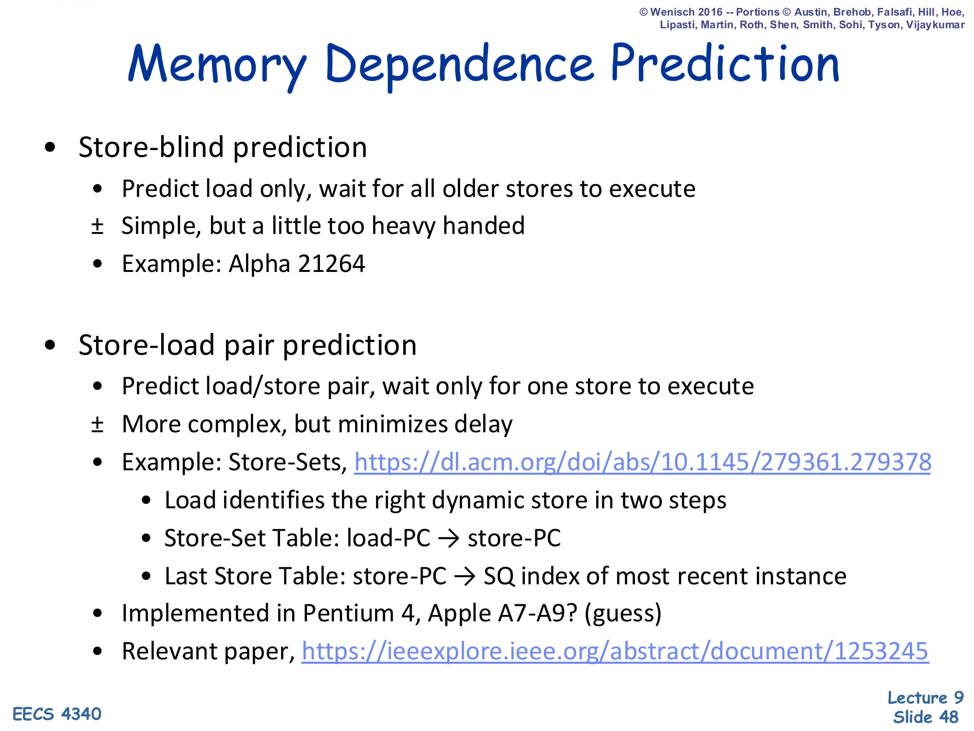
Memory Dependence Prediction
Show slide text
Memory Dependence Prediction
- Store-blind prediction
- Predict load only, wait for all older stores to execute
- ± Simple, but a little too heavy handed
- Example: Alpha 21264
- Store-load pair prediction
- Predict load/store pair, wait only for one store to execute
- ± More complex, but minimizes delay
- Example: Store-Sets (Chrysos & Emer, ISCA 1998)
- Load identifies the right dynamic store in two steps
- Store-Set Table: load-PC → store-PC
- Last Store Table: store-PC → SQ index of most recent instance
- Implemented in Pentium 4, Apple A7-A9? (guess)
- Relevant paper: IEEE Xplore
Two predictor designs realize intelligent load scheduling. Store-blind prediction (Alpha 21264) keeps a tiny table indexed by load PC and a single bit: “this load has caused violations before.” When such a load dispatches, it waits for every older store to execute — heavy-handed because most older stores don’t actually alias, but extremely simple. Store-load pair prediction (Chrysos & Emer’s Store-Sets, used in Pentium 4) is more precise: a Store-Set Table maps load PC to the store PC(s) it tends to depend on, and a Last Store Table maps each producing store PC to the SQ index of its most recent dynamic instance. A predicted-aliasing load only waits for that specific store to execute, not every older store. This recovers most of the speculative disambiguation benefit without the flush penalty, and is the foundation of modern memory-scheduling predictors. The slide cites the canonical 1998 ISCA paper and Chrysos’s later 2003 retrospective.
Summary (Memory Scheduling)
Show slide text
Summary
- Modern dynamic scheduling must support precise state
- A software sanity issue, not a performance issue
- Strategy: Writeback → Complete (OoO) + Retire (iO)
- Two basic designs
- P6: Tomasulo + re-order buffer, copy based register renaming
- ± Precise state is simple, but fast implementations are difficult
- R10K: implements true register renaming
- ± Easier fast implementations, but precise state is more complex
- P6: Tomasulo + re-order buffer, copy based register renaming
- Out-of-order memory operations
- Store queue: conservative load scheduling (iO wrt older stores)
- Load queue: opportunistic load scheduling (OoO wrt older stores)
- Intelligent memory scheduling: hybrid
The closing summary unifies the two halves of the lecture. The first half recapped the two OoO designs (P6 Tomasulo + ROB vs. R10K with true register renaming) and how each handles precise state. The second half built memory scheduling on top of either design. The store queue alone enables the conservative policy: loads stall for older stores’ addresses, so reordering happens only across loads and across stores but not across loads and stores. Adding a load queue plus violation detection enables the opportunistic (speculative) policy, where loads issue past unknown-address stores and recover via flush on misdisambiguation. The hybrid — intelligent scheduling with a dependence predictor — gives the best of both: opportunistic speed for non-aliasing loads, conservative ordering for the small set of loads predicted to alias. This completes the OoO execution story; L10 turns to branch prediction, the other major source of speculation.
Announcements (closing)

Show slide text
Announcements
- Project #4
- Due: milestone 3, 8-Apr-26
- Project meetings
- Mondays and Wednesdays during my office hours
- Mondays: CCDYMP, G13, GaPiChiXuXu, OoO
- Wednesdays: RISCy Whisky, SIX, UNI
- Mondays and Wednesdays during my office hours